
SLIDE 1
Definitions and examples Complexity of integration Poisson’s problem on a disc
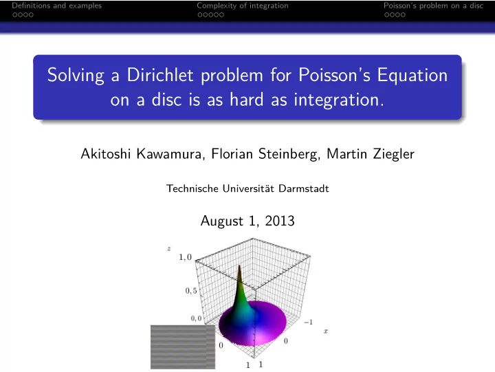
Solving a Dirichlet problem for Poisson’s Equation
- n a disc is as hard as integration.
Solving a Dirichlet problem for Poissons Equation on a disc is as - - PowerPoint PPT Presentation
Definitions and examples Complexity of integration Poissons problem on a disc Solving a Dirichlet problem for Poissons Equation on a disc is as hard as integration. Akitoshi Kawamura, Florian Steinberg, Martin Ziegler Technische
Definitions and examples Complexity of integration Poisson’s problem on a disc
Definitions and examples Complexity of integration Poisson’s problem on a disc
Definitions and examples Complexity of integration Poisson’s problem on a disc Reals
Definitions and examples Complexity of integration Poisson’s problem on a disc Real functions
1 Any H¨
2 The function
Definitions and examples Complexity of integration Poisson’s problem on a disc Real functions
1 f has a computable modulus of continuity. 2 the sequence of values of f on dyadic arguments is
1 it has a polynomial modulus of continuity. 2 there is a machine which, upon input d, 1n, returns a dyadic
Definitions and examples Complexity of integration Poisson’s problem on a disc An example
Definitions and examples Complexity of integration Poisson’s problem on a disc NP and #P
Definitions and examples Complexity of integration Poisson’s problem on a disc NP and #P
1 FP ⊆ #P. 2 FP = #P implies P = NP.
Definitions and examples Complexity of integration Poisson’s problem on a disc The complexity of integration
1 The indefinite integral over each polytime computable
2 FP = #P 3 The indefinite integral over each smooth, polytime
Definitions and examples Complexity of integration Poisson’s problem on a disc The complexity of integration
1..11 1..10 1..00 ... ... x
2−q(|x|)
Definitions and examples Complexity of integration Poisson’s problem on a disc Parameter integration
1 For any polytime computable f : [0, 1] × [0, 1] → R the
2 FP = #P.
Definitions and examples Complexity of integration Poisson’s problem on a disc
Definitions and examples Complexity of integration Poisson’s problem on a disc The greens function
1 FP = #P 2 The unique solution u is polytime computable whenever f is.
Definitions and examples Complexity of integration Poisson’s problem on a disc The greens function
Definitions and examples Complexity of integration Poisson’s problem on a disc Solving Poissons’s equation by integrating
Definitions and examples Complexity of integration Poisson’s problem on a disc Integrating by using the solution operator
Definitions and examples Complexity of integration Poisson’s problem on a disc