15. Poisson Processes In Lecture 4, we introduced Poisson arrivals - PowerPoint PPT Presentation

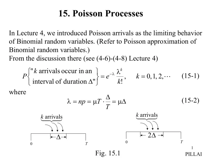
15. Poisson Processes In Lecture 4, we introduced Poisson arrivals as the limiting behavior of Binomial random variables. (Refer to Poisson approximation of Binomial random variables.) From the discussion there (see (4-6)-(4-8) Lecture 4) " k arrivals occur in an   λ k = − λ = (15-1) P e , k 0 , 1 , 2 , �   ∆ interval of duration " k !   where ∆ λ = = µ ⋅ = µ ∆ (15-2) np T T k arrivals � � � � � k arrivals � � � � � ∆ 2 ∆ T 0 T 0 1 Fig. 15.1 PILLAI

It follows that (refer to Fig. 15.1)  " arrivals occur in an k  = λ k (2 ) , − λ = 2 P e k 0, 1, 2, � ,   (15-3) ∆ interval of duration 2 " k !   since in that case ∆ 2 = µ ⋅ = µ ∆ = λ np T 2 2 . (15-4) 1 T From (15-1)-(15-4), Poisson arrivals over an interval form a Poisson random variable whose parameter depends on the duration of that interval. Moreover because of the Bernoulli nature of the underlying basic random arrivals, events over nonoverlapping intervals are independent. We shall use these two key observations to define a Poisson process formally. (Refer to Example 9-5, Text) Definition: X ( t ) = n (0, t ) represents a Poisson process if (i) the number of arrivals n ( t 1 , t 2 ) in an interval ( t 1 , t 2 ) of length λ t . t = t 2 – t 1 is a Poisson random variable with parameter Thus 2 PILLAI

λ k ( t ) = = − λ = = − t P { n ( t , t ) k } e , k 0 , 1 , 2 , � , t t t (15-5) 1 2 2 1 k ! and (ii) If the intervals ( t 1 , t 2 ) and ( t 3 , t 4 ) are nonoverlapping, then the random variables n ( t 1 , t 2 ) and n ( t 3 , t 4 ) are independent. P λ Since n (0, t ) ~ we have ( t ), (15-6) = = λ E [ X ( t )] E [ n ( 0 , t )] t and = = λ + λ (15-7) 2 2 2 2 E [ X ( t )] E [ n ( 0 , t )] t t . R XX ( t 1 t , ), To determine the autocorrelation function let t 2 > t 1 , 2 then from (ii) above n (0, t 1 ) and n ( t 1 , t 2 ) are independent Poisson λ λ t − random variables with parameters and respectively. t ( t ) 1 2 1 Thus = = λ − 2 E [ n ( 0 , t ) n ( t , t )] E [ n ( 0 , t )] E [ n ( t , t )] t ( t t ). (15-8) 1 1 2 1 1 2 1 2 1 3 PILLAI

But = − = − n ( t , t ) n ( 0 , t ) n ( 0 , t ) X ( t ) X ( t ) 1 2 2 1 2 1 and hence the left side if (15-8) can be rewritten as − = − 2 E [ X ( t ){ X ( t ) X ( t )}] R ( t , t ) E [ X ( t )]. (15-9) 1 2 1 1 2 1 XX Using (15-7) in (15-9) together with (15-8), we obtain = λ − + 2 2 R XX ( t , t ) t ( t t ) E [ X ( t )] 1 2 1 2 1 1 = λ + λ ≥ 2 (15-10) t t t , t t . 1 1 2 2 1 Similarly = λ + λ < 2 R XX ( t , t ) t t t , t t . (15-11) 1 2 2 1 2 2 1 Thus = λ + λ 2 R XX ( t , t ) t t min( t , t ). (15-12) 1 2 1 2 1 2 4 PILLAI

Poisson arrivals t t t 0 i 1 From (15-12), notice that X ( t ) the Poisson process X ( t ) does not represent a wide t sense stationary process. Y ( t ) + 1 t 1 t − 1 Define a binary level process Fig. 15.2 = − (15-13) X ( t ) Y ( t ) ( 1 ) that represents a telegraph signal (Fig. 15.2). Notice that the transition instants { t i } are random. (see Example 9-6, Text for the mean and autocorrelation function of a telegraph signal). Although X ( t ) does not represent a wide sense stationary process, 5 PILLAI

X ′ ( t ) its derivative does represent a wide sense stationary process. ( ⋅ d ) X ′ X ( t ) ( t ) dt Fig. 15.3 (Derivative as a LTI system) To see this, we can make use of Fig. 14.7 and (14-34)-(14-37). From there µ λ d ( t ) d t µ = = = λ ( t ) , a constant X (15-14) ′ dt dt X and  λ ≤ 2 ∂ t t t  R ( , ) t t 1 1 2 = =  R ( t , t ) 1 2 XX 1 2 ∂ ′ XX t λ + λ > 2  t t t  2 1 1 2 = λ + λ − 2 t U t ( t ) (15-15) 1 1 2 and ∂ R ( t , t ) = = λ + λ δ − 2 R ( t , t ) 1 2 ( t t ). ′ X X (15-16) 1 2 1 2 ∂ ′ ′ 6 X X t 1 PILLAI

X ′ ( t ) From (15-14) and (15-16) it follows that is a wide sense stationary process. Thus nonstationary inputs to linear systems can lead to wide sense stationary outputs, an interesting observation. • Sum of Poisson Processes: If X 1 ( t ) and X 2 ( t ) represent two independent Poisson processes, then their sum X 1 ( t ) + X 2 ( t ) is also a Poisson process with λ + λ parameter (Follows from (6-86), Text and the definition ( ) t . 1 2 of the Poisson process in (i) and (ii)). • Random selection of Poisson Points: t , t , � , t , � Let represent random arrival points associated 1 2 i λ t , with a Poisson process X ( t ) with parameter and associated with � � each arrival point, t define an independent t t t 1 2 i Bernoulli random Fig. 15.4 variable N i , where = = = = = − 7 P ( N 1 ) p , P ( N 0 ) q 1 p . (15-17) i i PILLAI

Define the processes X ( t ) X ( t ) ∑ ∑ = = − = − Y ( t ) N ; Z ( t ) ( 1 N ) X ( t ) Y ( t ) (15-18) i i = = i 1 i 1 we claim that both Y ( t ) and Z ( t ) are independent Poisson processes λ λ with parameters and respectively. pt qt Proof: ∞ ∑ = = = = (15-19) Y ( t ) P { Y ( t ) k | X ( t ) n } P { X ( t ) n )}. = n k n ∑ = But given X ( t ) = n, we have so that Y ( t ) N ~ B ( n , p ) i = i 1 ( ) = = = − ≤ ≤ k n k P Y t { ( ) k X t | ( ) n } p q , 0 k n , (15-20) n k and λ n ( t ) = = − λ t P X t { ( ) n } e . (15-21) n ! Substituting (15-20)-(15-21) into (15-19) we get 8 PILLAI

− λ k t ∞ ∞ p e ∑ ∑ − n n k λ λ − λ − = = t k n k ( t ) = λ k ( q t ) P Y t { ( ) k } e p q ( t ) n ! − − ( n k )! ! k n ! ( n k )! k ! = � = � �� � n k n k λ q t e − − λ (1 q ) t λ k e ( pt ) = λ = − λ = k pt ( pt ) e , k 0, 1, 2, � k ! k ! (15-22) λ ~ ( P pt ). More generally, = = = = − = P Y t { ( ) k Z t , ( ) m } P Y t { ( ) k X t , ( ) Y t ( ) m } = = = + P Y t { ( ) k X t , ( ) k m } = = = + = + P Y t { ( ) k X t | ( ) k m P X t } { ( ) k m } + λ k m λ n λ n ( t ) ( pt ) ( qt ) ( ) = ⋅ − λ = − λ − λ k m t pt qt p q e e e + k m k + ( k m )! k ! m ! ����� �� �� � = = P Y t ( ( ) k ) P Z ( ( t ) m ) = = = P Y t { ( ) k P Z t } { ( ) m }, 9 (15-23) PILLAI

which completes the proof. Notice that Y ( t ) and Z ( t ) are generated as a result of random Bernoulli selections from the original Poisson process X ( t ) (Fig. 15.5), where each arrival gets tossed over to either Y ( t ) with λ Y ( t ) ~ P ( pt ) probability p or to Z ( t ) with t probability q . Each such p p p p sub-arrival stream is also a Poisson process. Thus λ X ( t ) ~ P ( t ) random selection of Poisson t points preserve the Poisson nature of the resulting q q processes. However, as we λ Z ( t ) ~ P ( qt ) shall see deterministic t selection from a Poisson Fig. 15.5 process destroys the Poisson property for the resulting processes. 10 PILLAI

Inter-arrival Distribution for Poisson Processes τ 2 nd n th Let denote the time interval (delay) 1 I st arrival arrival to the first arrival from any fixed point � t t 0 . To determine the probability 0 t τ t t t distribution of the random variable 1 1 2 n τ , Fig. 15.6 we argue as follows: Observe that 1 τ > " t " the event is the same as “ n ( t 0 , t 0 + t ) = 0”, or the complement 1 τ ≤ event is the same as the event “ n ( t 0 , t 0 + t ) > 0” . " t " 1 τ Hence the distribution function of is given by 1 ∆ = τ ≤ = > = + > F ( ) t P { t } P X t { ( ) 0} P n t t { ( , t ) 0} τ 1 0 0 1 − λ = − + = = − t (15-24) 1 P n t t { ( , t ) 0} 1 e 0 0 (use (15-5)), and hence its derivative gives the probability density τ function for to be 1 dF ( ) t τ − λ = = λ ≥ t f ( ) t e , t 0 1 (15-25) τ dt 1 τ i.e., is an exponential random variable with parameter λ 1 11 τ = λ so that E ( 1 ) 1 / . PILLAI