The Model Problem Scientific Computing I 2D Poisson Equation on - PDF document

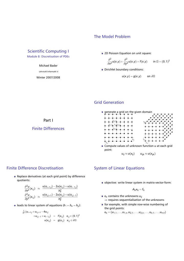
The Model Problem Scientific Computing I 2D Poisson Equation on unit square: Module 8: Discretisation of PDEs ∂ x 2 u ( x , y )+ ∂ 2 ∂ 2 in Ω = ( 0 , 1 ) 2 ∂ y 2 u ( x , y ) = f ( x , y ) Michael Bader Dirichlet boundary conditions: Lehrstuhl Informatik V u ( x , y ) = g ( x , y ) on ∂ Ω Winter 2007/2008 Grid Generation generate a grid on the given domain Part I x i,j+1 h y x i−1,j x i,j x i+1,j Finite Differences x i,j−1 h y h z h x h x Compute values of unknown function u at each grid point: u ij ≈ u ( x ij ) u ijk ≈ u ( x ijk ) Finite Difference Discretisation System of Linear Equations Replace derivatives (at each grid point) by difference quotients: objective: write linear system in matrix-vector-form: ∂ 2 u u ( x i + 1 , j ) − 2 u ( x i , j )+ u ( x i − 1 , j ) ∂ x 2 ( x i , j ) ≈ A h x h = f h h 2 x ∂ 2 u u ( x i , j + 1 ) − 2 u ( x i , j )+ u ( x i , j − 1 ) x h contains the unknowns u ij ∂ y 2 ( x i , j ) ≈ h 2 y ⇒ requires sequentialisation of the unknowns for example, with simple row-wise numbering of leads to linear system of equations ( h := h x = h y ): the grid points: � 1 u i + 1 , j + u i , j + 1 − 4 u i , j x h = ( u 1 , 1 ,..., u 1 , n , u 2 , 1 ,..., u 2 , n ,..., u n , 1 ,..., u n , n ) h 2 � x i , j ∈ ( 0 , 1 ) 2 + u i , j − 1 + u i − 1 , j = f ( x i , j ) u ( x i , j ) = g ( x i , j ) x i , j ∈ ∂ Ω

System of Linear Equations (2) Stencil Notation A h is a sparse matrix (five-diagonal) illustrate matrix structure as a discretisation stencil A h is a block-tridiagonal matrix: represents one line of the matrix   matrix elements placed according to their B h I corresponding geometrical position ... ...   A h = 1 I   stencils for the Poisson equation ( h 2 factors   ... ... h 2   I   ignored): I B h   1 B h = tridiag ( 1 , − 4 , 1 ) � � 1 D : 1 − 2 1 2 D : 1 − 4 1   I the identity matrix 1 boundary values to right-hand side Accuracy for 5-point Poisson stencil; order of accuracy: � u h − u � = O ( h 2 ) = O ( N − 2 ) Part II curse of dimension: for that, we need O ( N d ) points Finite Element Methods Possibilities of an improvement: use higher-order discretisation via higher order terms of Taylor series leads to larger stencils (involving more neighbouring grid points) use locally refined ( adaptive ) grids Finite Elements – Main Ingredients Choose Test and Ansatz Space compute a function as numerical solution; 1 search in a function space W h : search for solution functions u h of the form u h = ∑ u h = ∑ u j ϕ j ( x ) , span { ϕ 1 ,..., ϕ J } = W h u j ϕ j ( x ) j j solve weak form of PDE to reduce regularity 2 the basis (ansatz) functions ϕ j ( x ) build a vector properties space (or function space) W h � � u ′′ = f v ′ u ′ dx = span { ϕ 1 ,..., ϕ J } = W h − → vf dx the “best” solution u h in this function space is choose basis functions with local support , e.g.: 3 wanted ϕ j ( x i ) = δ ij

Example: Nodal Basis Weak Forms and Weak Solutions  1 h ( x − x i − 1 ) x i − 1 < x < x i   1 consider a PDE Lu = f (e.g. Lu = ∆ u ) ϕ i ( x ) := h ( x i + 1 − x ) x i < x < x i + 1   transformation to the weak form : 0 otherwise � � � Lu , v � = vLu dx = vf dx = � f , v � ∀ v ∈ V 1 V a certain class of functions 0,8 “real solution” u also solves the weak form 0,6 � Lu , v � a bilinear form ; often written as: 0,4 a ( u , v ) = � f , v � ∀ v ∈ V 0,2 0 0 0,2 0,4 0,6 0,8 1 x Weak Form of the Poisson Equation Weak Form of the Poisson Equation (2) Poisson equation with Dirichlet conditions: Poisson equation with Dirichlet conditions: − ∆ u = f in Ω , u = 0 on δ Ω − ∆ u = f in Ω , u = 0 on δ Ω weak form: � � transformed into weak form: − Ω v ∆ u d Ω = Ω vf d Ω ∀ v � � Ω ∇ v · ∇ u d Ω = Ω vf d Ω ∀ v apply Green’s formula: � � � weaker requirements for a solution u : − Ω v ∆ u d Ω = Ω ∇ v · ∇ u d Ω − ∂ Ω v · ∇ uds twice differentiabale → first derivative integrable remember use of nodal basis: availability of first vs. choose functions v such that v = 0 on ∂ Ω : second derivative! � � Ω ∇ v · ∇ u d Ω = Ω vf d Ω ∀ v Choose Test and Ansatz Space Choose Test and Ansatz Space (2) choose a basis { ψ i } of the test space V search for solutions u h in a function space W h : then: if all basis functions ψ i satisfy u h = ∑ u j ϕ j ( x ) � � � � ∑ ψ i L u j ϕ j ( x ) dx = ψ i f dx ∀ ψ i j j where span { ϕ j } = W h (“ansatz space”) then all v ∈ V satisfy the equation insert into weak solution leads to system of equations for unknowns u j � � � � ∑ vL u j ϕ j ( x ) dx = vf dx ∀ v ∈ V (one equation per test basis function ψ i ) j V is often chosen to be identical to W h (Ritz-Galerkin method)

Discretisation – Finite Elements Example Problem: Poisson 1D L linear ⇒ system of linear equations in 1D: u ′′ ( x ) = f ( x ) on Ω = ( 0 , 1 ) , � � � � hom. Dirichlet boundary cond.: u ( 0 ) = u ( 1 ) = 0 ∑ ψ i L ϕ j ( x ) dx u j = ψ i f dx ∀ ψ i weak form: j � �� � =: A ij � 1 � 1 0 v ′ ( x ) · u ′ ( x ) dx = 0 v ( x ) f ( x ) dx ∀ v aim: make matrix A sparse → most A ij = 0 approach: local basis functions on a discretisation compuational grid: grid x i = ih , (for i = 1 ,..., n − 1); mesh size h = 1 / n ψ j , ϕ j zero everywhere except in grid cells adjacent V = W : piecewise linear functions to grid point x j (on intervals [ x i , x i + 1 ] ) A ij = 0, if ψ i and ϕ j don’t overlap Nodal Basis Nodal Basis – System of Equations  1 h ( x − x i − 1 ) x i − 1 < x < x i   stiffness matrix: 1 ϕ i ( x ) := h ( x i + 1 − x ) x i < x < x i + 1    2 − 1  0 otherwise ...   1 − 1 2     ... ... h   − 1 1   − 1 2 0,8 right hand sides (assume f ( x ) = α ∈ R ): 0,6 � 1 � 1 0,4 0 ϕ i ( x ) f ( x ) dx = 0 ϕ i ( x ) α dx = α h 0,2 system of equations very similar to finite differences 0 0 0,2 0,4 0,6 0,8 1 x Element Stiffness Matrices Element Stiffness Matrices (2) leads to local stiffness matrices for each element: domain Ω splitted into finite elements Ω ( k ) : � Ω = Ω ( 1 ) ∪ Ω ( 2 ) ∪···∪ Ω ( n ) Ω ( k ) ∇ φ i · ∇ φ j dx � �� � =: A ( k ) observation: basis functions are defined ij element-wise and respective element systems: � b � c � b use: a f ( x ) dx = a f ( x ) dx + c f ( x ) dx A ( k ) x = b ( k ) element-wise evaluation of the integrals: � � = ∑ accumulate to obtain global system: Ω ∇ v · ∇ u dx Ω ( k ) ∇ v · ∇ u dx k x = ∑ A ( k ) b ( k ) ∑ � � = ∑ Ω vf dx Ω ( i ) vf dx k k � �� � i =: A

Element Stiffness Matrices (3) Example: 1D Poisson Ω = [ 0 , 1 ] splitted into Ω ( k ) = [ x k − 1 , x k ] Some comments on notation: nodal basis; leads to element stiffness matrix: assume: 1D problem, n elements (i.e. intervals) � � 1 − 1 in each element only two basis functions are A ( k ) = − 1 1 non-zero! hence, almost all A ( k ) are zero: consider only two elements: ij �     A ( k ) 1 − 1 0 0 0 0 = Ω ( k ) ∇ φ i · ∇ φ j dx ij A ( 1 ) + A ( 2 ) = − 1 1 0  + 0 1 − 1    only 2 × 2 elements of A ( k ) are non-zero 0 0 0 0 − 1 1 therefore convention to omit zero columns/rows in stencil notation: ⇒ leaves only unknowns that are in Ω ( k ) 1 ∗ ] + [ 1 ∗ − 1 ] → [ − 1 [ − 1 2 − 1 ] Example: 2D Poisson Example: 2D Poisson (2) − ∆ u = f on domain Ω = [ 0 , 1 ] 2 splitted into Ω ( i , j ) = [ x i − 1 , x i ] × [ x j − 1 , x j ] leads to element stiffness matrix: bilinear basis functions   − 1 − 1 2 − 1 2 2   ϕ ij ( x , y ) = ϕ i ( x ) ϕ j ( y ) − 1 − 1 2 − 1 A ( k ) =   2 2   − 1 − 1  − 1 2  “pagoda” functions 2 2   − 1 − 1 − 1 2 2 2 accumulation leads to 9-point stencil   − 1 − 1 − 1   − 1 8 − 1   − 1 − 1 − 1 Typical workflow Time-Dependent Problems choose elements: 1 Example: 1D Heat Equation quadratic or cubic cells u t = u xx + f on domain Ω = [ 0 , 1 ] for t ∈ [ 0 , t end ] triangles (structured, unstructured) spatial discretisation: weak form tetrahedra, etc. set up basis functions for each element Ω ( k ) ; 2 � � � vu t dx = vu xx dx + vf dx for example, at all nodes x i ∈ Ω ( k ) � � � � � ∂ ϕ i ( x i ) = 1 vu dx = vu xx dx + vf dx ∂ t ϕ i ( x j ) = 0 for all j � = i spatial discretisation – finite elements: for element stiffness matrix, compute all 3 ∂ ∂ t ( M h u h ) = A h u h + f h � A ( k ) = Ω ( k ) ϕ i L ϕ j d Ω ij M h : mass matrix, A h : stiffness matrix, u h = u h ( t ) accumulate global stiffness matrix 4