
SLIDE 1
1
Ascription and Achievement in Occupational Attainment in Comparative Perspective: a comparison of 42 nations, 1900-2000
Harry B.G. Ganzeboom Donald J. Treiman
Russell Sage University Working Group on Social Inequality University of California-Los Angeles January 25-26 2007
2
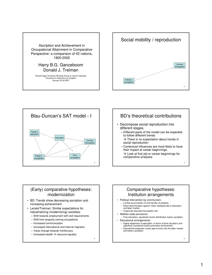
Social mobility / reproduction
Father’s
- ccupation
Current Occupation
3
Blau-Duncan’s SAT model - I
Father’s education Father’s
- ccupation
Education First
- ccupation
Current Occupation
4
BD’s theoretical contributions
- Decompose social reproduction into
different stages.
– Different parts of the model can be expected to follow different trends There is no expectation about trends in social reproduction – Contextual influences are most likely to have their impact at career beginnings. Look at first job or career beginnings for comparative analyses
5
(Early) comparative hypotheses: modernization
- BD: Trends show decreasing ascription and
increasing achievement
- Lenski/Treiman: Similar expectations for
industrializing (modernizing) societies:
– Shift towards employment with skill requirements – Shift from property owning occupations – Increased communication – Increased international and internal migration – Value change towards meritocracy – Increased wealth resource equality
6
Comparative hypotheses: Institution arrangements
- Political intervention by communism:
– Limited accumulation of and transfer of property. – Direct discrimination against ‘class’ backgrounds in education and labor market. – Organized education/occupation link.
- Welfare state provisions:
– Free education, equalized income distribution lowers ascription
- Educational arrangements:
– Higher dispersion of education, in terms of level (duration) and specificity (vocational tracks) promotes achievement – Educational expansion raises age of entry into the labor market and lowers ascription