[PDF] - So far: features and filters Motion magnification Transforming PDF Document

SLIDE 1

CS 376: Computer Vision - lecture 7 2/7/2018 1

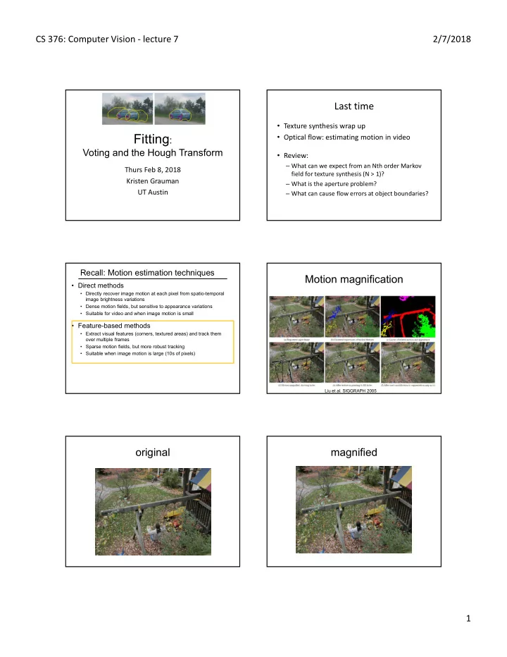
Fitting:

Voting and the Hough Transform

Thurs Feb 8, 2018 Kristen Grauman UT Austin

Last time

Texture synthesis wrap up
Optical flow: estimating motion in video
Review:

– What can we expect from an Nth order Markov field for texture synthesis (N > 1)? – What is the aperture problem? – What can cause flow errors at object boundaries?

Recall: Motion estimation techniques

Direct methods
Directly recover image motion at each pixel from spatio-temporal

image brightness variations

Dense motion fields, but sensitive to appearance variations
Suitable for video and when image motion is small
Feature-based methods
Extract visual features (corners, textured areas) and track them
ver multiple frames
Sparse motion fields, but more robust tracking
Suitable when image motion is large (10s of pixels)

Motion magnification

Liu et al. SIGGRAPH 2005

riginal

magnified

SLIDE 2

CS 376: Computer Vision - lecture 7 2/7/2018 2

Motion magnification

http://people.csail.mit.edu/mrub/vidmag/ Hao-Yu Wu, Michael Rubinstein, Eugene Shih, John Guttag, Frédo Durand, William T.

Freeman. Eulerian Video Magnification for Revealing Subtle Changes in the World ACM

Transactions on Graphics, Volume 31, Number 4 (Proc. SIGGRAPH), 2012

So far: features and filters

Transforming images; gradients, textures, edges, flow

Now: Fitting

Want to associate a model with observed features

[Fig from Marszalek & Schmid, 2007]

For example, the model could be a line, a circle, or an arbitrary shape.

Fitting: Main idea

Choose a parametric model to represent a

set of features

Membership criterion is not local
Can’t tell whether a point belongs to a given model just by

looking at that point

Three main questions:
What model represents this set of features best?
Which of several model instances gets which feature?
How many model instances are there?
Computational complexity is important
It is infeasible to examine every possible set of parameters

and every possible combination of features

Slide credit: L. Lazebnik

Case study: Line fitting

Why fit lines?

Many objects characterized by presence of straight lines

Wait, why aren’t we done just by running edge detection?
Extra edge points (clutter),

multiple models:

– which points go with which line, if any?

Only some parts of each line

detected, and some parts are missing:

– how to find a line that bridges missing evidence?

Noise in measured edge

points, orientations:

– how to detect true underlying parameters?

Difficulty of line fitting

SLIDE 3

CS 376: Computer Vision - lecture 7 2/7/2018 3

Voting

It’s not feasible to check all combinations of features by

fitting a model to each possible subset.

Voting is a general technique where we let the features

vote for all models that are compatible with it.

– Cycle through features, cast votes for model parameters. – Look for model parameters that receive a lot of votes.

Noise & clutter features will cast votes too, but typically

their votes should be inconsistent with the majority of “good” features.

Fitting lines: Hough transform

Given points that belong to a line, what

is the line?

How many lines are there?
Which points belong to which lines?
Hough Transform is a voting

technique that can be used to answer all of these questions. Main idea:

1. Record vote for each possible line
n which each edge point lies.
2. Look for lines that get many votes.

Finding lines in an image: Hough space

Connection between image (x,y) and Hough (m,b) spaces

A line in the image corresponds to a point in Hough space
To go from image space to Hough space:

– given a set of points (x,y), find all (m,b) such that y = mx + b

x y m b m0 b0

image space Hough (parameter) space

Slide credit: Steve Seitz

Finding lines in an image: Hough space

Connection between image (x,y) and Hough (m,b) spaces

A line in the image corresponds to a point in Hough space
To go from image space to Hough space:

– given a set of points (x,y), find all (m,b) such that y = mx + b

What does a point (x0, y0) in the image space map to?

x y m b

image space Hough (parameter) space

– Answer: the solutions of b = -x0m + y0 – this is a line in Hough space

x0 y0

Slide credit: Steve Seitz

Finding lines in an image: Hough space

What are the line parameters for the line that contains both (x0, y0) and (x1, y1)?

It is the intersection of the lines b = –x0m + y0 and

b = –x1m + y1 x y m b

image space Hough (parameter) space

x0 y0

b = –x1m + y1 (x0, y0) (x1, y1)

Finding lines in an image: Hough algorithm

How can we use this to find the most likely parameters (m,b) for the most prominent line in the image space?

Let each edge point in image space vote for a set of

possible parameters in Hough space

Accumulate votes in discrete set of bins*; parameters with

the most votes indicate line in image space.

x y m b

image space Hough (parameter) space

SLIDE 4

CS 376: Computer Vision - lecture 7 2/7/2018 4

Polar representation for lines

: perpendicular distance from line to origin : angle the perpendicular makes with the x-axis

Point in image space  sinusoid segment in Hough space

d y x     sin cos

d



[0,0]

d 

x

y

Issues with usual (m,b) parameter space: can take on infinite values, undefined for vertical lines.

Image columns Image rows

Hough transform algorithm

Using the polar parameterization: Basic Hough transform algorithm

1. Initialize H[d, ]=0
2. for each edge point I[x,y] in the image

for  = [min to max ] // some quantization H[d, ] += 1

3. Find the value(s) of (d, ) where H[d, ] is maximum
4. The detected line in the image is given by

H: accumulator array (votes)

d 

Time complexity (in terms of number of votes per pt)?

d y x     sin cos

Source: Steve Seitz

  sin cos y x d  

Example: What was the shape?

Circle : Square :

d 

Example: Hough transform for straight lines

Which line generated this peak?

Original image Canny edges Vote space and top peaks

d 

Decode the vote space.

SLIDE 5

CS 376: Computer Vision - lecture 7 2/7/2018 5

Showing longest segments found

Impact of noise on Hough

Image space edge coordinates Votes

 x y d

What difficulty does this present for an implementation? Image space edge coordinates Votes

Impact of noise on Hough

Here, everything appears to be “noise”, or random edge points, but we still see peaks in the vote space.

Extensions

Extension 1: Use the image gradient

1. same 2. for each edge point I[x,y] in the image

 = gradient at (x,y)

H[d, ] += 1 3. same 4. same

(Reduces degrees of freedom) Extension 2

give more votes for stronger edges

Extension 3

change the sampling of (d, ) to give more/less resolution

Extension 4

The same procedure can be used with circles, squares, or any
ther shape

  sin cos y x d  

Extensions

Extension 1: Use the image gradient

1. same 2. for each edge point I[x,y] in the image compute unique (d, ) based on image gradient at (x,y) H[d, ] += 1 3. same 4. same

(Reduces degrees of freedom) Extension 2

give more votes for stronger edges (use magnitude of gradient)

Extension 3

change the sampling of (d, ) to give more/less resolution

Extension 4

The same procedure can be used with circles, squares, or any
ther shape…

Source: Steve Seitz

Hough transform for circles

For a fixed radius r, unknown gradient direction
Circle: center (a,b) and radius r

2 2 2

) ( ) ( r b y a x

i i

   

Image space Hough space

a b

SLIDE 6

CS 376: Computer Vision - lecture 7 2/7/2018 6

Hough transform for circles

For a fixed radius r, unknown gradient direction
Circle: center (a,b) and radius r

2 2 2

) ( ) ( r b y a x

i i

   

Image space Hough space Intersection: most votes for center occur here.

Hough transform for circles

For an unknown radius r, unknown gradient direction
Circle: center (a,b) and radius r

2 2 2

) ( ) ( r b y a x

i i

   

Hough space Image space

b a r

?

Hough transform for circles

For an unknown radius r, unknown gradient direction
Circle: center (a,b) and radius r

2 2 2

) ( ) ( r b y a x

i i

   

Hough space Image space

b a r

Hough transform for circles

For an unknown radius r, known gradient direction
Circle: center (a,b) and radius r

2 2 2

) ( ) ( r b y a x

i i

   

Hough space Image space

θ

x

Hough transform for circles

For every edge pixel (x,y) : For each possible radius value r: For each possible gradient direction θ: // or use estimated gradient at (x,y) a = x + r cos(θ) // column b = y - r sin(θ) // row H[a,b,r] += 1 end end

Check out online demo : http://www.markschulze.net/java/hough/

Time complexity per edge pixel?

Original Edges

Example: detecting circles with Hough

Votes: Penny Note: a different Hough transform (with separate accumulators) was used for each circle radius (quarters vs. penny).

SLIDE 7

CS 376: Computer Vision - lecture 7 2/7/2018 7

Original Edges

Example: detecting circles with Hough

Votes: Quarter Combined detections

Coin finding sample images from: Vivek Kwatra

Example: iris detection

Hemerson Pistori and Eduardo Rocha Costa

http://rsbweb.nih.gov/ij/plugins/hough-circles.html Gradient+threshold Hough space (fixed radius) Max detections

Example: iris detection

An Iris Detection Method Using the Hough Transform and Its Evaluation for

Facial and Eye Movement, by Hideki Kashima, Hitoshi Hongo, Kunihito Kato, Kazuhiko Yamamoto, ACCV 2002.

Voting: practical tips

Minimize irrelevant tokens first
Choose a good grid / discretization
Vote for neighbors, also (smoothing in

accumulator array)

Use direction of edge to reduce parameters by 1
To read back which points voted for “winning”

peaks, keep tags on the votes.

Too coarse Too fine

?

Hough transform: pros and cons

Pros

All points are processed independently, so can cope with
cclusion, gaps
Some robustness to noise: noise points unlikely to

contribute consistently to any single bin

Can detect multiple instances of a model in a single pass

Cons

Complexity of search time increases exponentially with

the number of model parameters

Non-target shapes can produce spurious peaks in

parameter space

Quantization: can be tricky to pick a good grid size

Generalized Hough Transform

Model image Vote space Novel image x x x x x

Now suppose those colors encode gradient directions…

What if we want to detect arbitrary shapes?

Intuition:

Ref. point

Displacement vectors

SLIDE 8

CS 376: Computer Vision - lecture 7 2/7/2018 8

Define a model shape by its boundary points

and a reference point.

[Dana H. Ballard, Generalizing the Hough Transform to Detect Arbitrary Shapes, 1980]

x a

p1

θ

p2

θ

At each boundary point, compute displacement vector: r = a – pi. Store these vectors in a table indexed by gradient orientation θ.

Generalized Hough Transform

Offline procedure:

Model shape

θ θ

… … …

p1

θ θ

For each edge point:

Use its gradient orientation θ

to index into stored table

Use retrieved r vectors to

vote for reference point

Generalized Hough Transform

Detection procedure:

Assuming translation is the only transformation here, i.e., orientation and scale are fixed.

x

θ θ

Novel image

θ θ

… … …

θ

xx xx

Generalized Hough for object detection

Instead of indexing displacements by gradient
rientation, index by matched local patterns.
B. Leibe, A. Leonardis, and B. Schiele, Combined Object Categorization and

Segmentation with an Implicit Shape Model, ECCV Workshop on Statistical Learning in Computer Vision 2004 training image “visual codeword” with displacement vectors

Source: L. Lazebnik

Instead of indexing displacements by gradient
rientation, index by “visual codeword”
B. Leibe, A. Leonardis, and B. Schiele, Combined Object Categorization and

Segmentation with an Implicit Shape Model, ECCV Workshop on Statistical Learning in Computer Vision 2004 test image

Source: L. Lazebnik