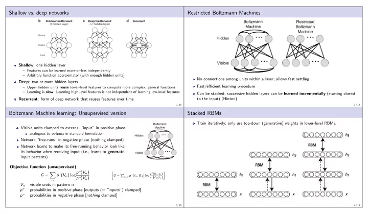
Shallow vs. deep networks Restricted Boltzmann Machines Shallow : - - PowerPoint PPT Presentation

Shallow vs. deep networks

Shallow: one hidden layer

– Features can be learned more-or-less independently – Arbitrary function approximator (with enough hidden units)

Deep: two or more hidden layers

– Upper hidden units reuse lower-level features to compute more complex, general functions – Learning is slow: Learning high-level features is not independent of learning low-level features

Recurrent: form of deep network that reuses features over time

1 / 18

Boltzmann Machine learning: Unsupervised version

Visible units clamped to external “input” in positive phase

analogous to outputs in standard formulation

Network “free-runs” in negative phase (nothing clamped) Network learns to make its free-running behavior look like its behavior when receiving input (i.e., learns to generate input patterns) Objective function (unsupervised) G =

• α

p+(Vα) logp+(Vα) p−(Vα)

• G =

α,β p+

Iα, Oβ

• log

p+(Oβ|Iα) p−(Oβ|Iα)

• Vα

visible units in pattern α p+ probabilities in positive phase [outputs (= “inputs”) clamped] p− probabilities in negative phase [nothing clamped]

2 / 18

Restricted Boltzmann Machines

No connections among units within a layer; allows fast settling Fast/efficient learning procedure Can be stacked; successive hidden layers can be learned incrementally (starting closest to the input) (Hinton)

3 / 18

Stacked RBMs

Train iteratively; only use top-down (generative) weights in lower-level RBMs.

4 / 18

Deep autoencoder (Hinton & Salakhutdinov, 2006, Science)

5 / 18

Face reconstructions (Hinton & Salakhutdinov, 2006)

Top: Original images in test set Middle: Network reconstructions (30-unit bottleneck) Bottom: PCA reconstructions (30 components)

6 / 18

Digit reconstructions (Hinton & Salakhutdinov, 2006)

PCA reconstructions (2 components) Network reconstructions (2-unit bottleneck)

7 / 18

Document retrieval (Hinton & Salakhutdinov, 2006)

Latent Semantic Analysis (2D) Network (2D)

8 / 18

Deep learning with back-propagation

Sigmoid function leads to extremely small derivatives for early layers (due to asympototes) Linear units preserve derivatives but cannot alter similarity structure Rectified linear units (ReLUs) preserve derivatives but impose (limited) non-linearity

Net input

Often applied with dropout: On any given trial, only a random subset

• f units (e.g., half) actually work (i.e., produce output if input > 0).

9 / 18

Online simulator

playground.tensorflow.org

10 / 18

Deep learning with back-propagation: Technical advances

Huge datasets available via the internet (“big data”) Application of GPUs (Graphics Processing Units) for very efficient 2D image processing

Krizhevsky, Sutskever, and Hinton (2012, NIPS)

11 / 18

What does a deep network learn?

Feedfoward network: 40 inputs to 40

• utputs via 6 hidden layers (of size 40)

Random input patterns map to random output patterns (n = 100)

Compute pairwise similarities of representations at each hidden layer Compare pairwise similarities of hidden representations to those among input

• r output representations

(⇒ Representational Similarity Analysis)

Network gradually transforms from input similarity to output similarity

12 / 18

Promoting generalization

Prevent overfitting by constraining network in a general way

– weight decay, cross-validation

Train on so much data that it’s not possible to overfit

– Including fabricating new data by transforming existing data in a way that you know the network must generalize over (e.g., viewpoint, color, lighting transformations) – Can also train an adversarial network to generate examples that produce high error

Constrain structure of network in a way that forces a specific type of generalization

– Temporal invariance Long short-term memory networks (LSTMs) Time-delay neural networks (TDNNs) – Position invariance Convolutional neural networks (CNNs)

13 / 18

Long short-term memory networks (LSTMs)

Learning long-distance dependencies requires preserving information over multiple time steps Conventential networks (e.g., SRNs) must learn to do this LSTM networks use much more complex “units” that intrinsically preserve and manipulate information

14 / 18

Long short-term memory networks (LSTMs)

15 / 18

Time-delay neural networks (TDNNs)

16 / 18

Convolutional neural networks (CNNs)

Hidden units organized into feature maps (each using weight sharing to enforce identical receptive fields) Subsequent layer “pools” across features at similar locations (e.g., MAX function)

17 / 18

Deep learning with back-propagation: Technical advances

Huge datasets available via the internet (“big data”) Application of GPUs (Graphics Processing Units) for very efficient 2D image processing

Krizhevsky, Sutskever, and Hinton (2012, NIPS)

18 / 18