
SLIDE 1
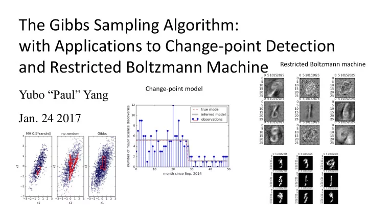
The Gibbs Sampling Algorithm: with Applications to Change-point Detection and Restricted Boltzmann Machine
Yubo “Paul” Yang
- Jan. 24 2017
Change-point model Restricted Boltzmann machine
with Applications to Change-point Detection and Restricted Boltzmann - - PowerPoint PPT Presentation
The Gibbs Sampling Algorithm: with Applications to Change-point Detection and Restricted Boltzmann Machine Restricted Boltzmann machine Change-point model Yubo Paul Yang Jan. 24 2017 Introduction: History Stuart Geman Donald Geman @
Change-point model Restricted Boltzmann machine
Donald Geman @ Johns Hopkins
Literature from UIUC
from Northwestern Stuart Geman @ Brown
UMich
Neurophysiology from Dartmouth
Mathematics from MIT
i.e. Acceptance = 1
Basic version: Block version: Collapsed version: Samplers within Gibbs:
Basic Gibbs sampling from bivariate Normal
Example inspired by: MCMC: The Gibbs Sampler , The Clever Machine, https://theclevermachine.wordpress.com/2012/1 1/05/mcmc-the-gibbs-sampler/
Q0/ How to sample 𝑦 from standard normal distribution Ɲ(𝜈 = 0, 𝜏 = 1)?
Example inspired by: MCMC: The Gibbs Sampler , The Clever Machine, https://theclevermachine.wordpress.com/2012/1 1/05/mcmc-the-gibbs-sampler/
𝑄 𝑦1, 𝑦2 = Ɲ(𝜈1, 𝜈2, Σ) = 1 2𝜌𝜏1𝜏2 1 − 𝜍2 𝑓𝑦𝑞 − 𝑨 2(1 − 𝜍2) Q0/ How to sample 𝑦 from standard normal distribution Ɲ(𝜈 = 0, 𝜏 = 1)? A0/ np.random.randn() samples from P(x) =
1 2𝜌𝜏2 exp[− 𝑦−𝜈 2 2𝜏2 ].
Bivariate normal distribution is the generalization of the normal distribution to two variables:
For simplicity, let 𝜈1 = 𝜈2 = 0, and 𝜏1 = 𝜏2 = 1 then:
Example inspired by: MCMC: The Gibbs Sampler , The Clever Machine, https://theclevermachine.wordpress.com/2012/1 1/05/mcmc-the-gibbs-sampler/
𝑄 𝑦1, 𝑦2 = Ɲ(𝜈1, 𝜈2, Σ) = 1 2𝜌𝜏1𝜏2 1 − 𝜍2 𝑓𝑦𝑞 − 𝑨 2(1 − 𝜍2) Σ = 𝜏1 𝜍 𝜍 𝜏2 where 𝑨 = 𝑦1 − 𝜈1 2 𝜏1
2
− 2𝜍 𝑦1 − 𝜈1 𝑦2 − 𝜈2 𝜏1𝜏2 + 𝑦2 − 𝜈2 2 𝜏2
2
and l𝑜 𝑄 𝑦1, 𝑦2 = − 𝑦1
2 − 2𝜍𝑦1𝑦2 + 𝑦2 2
2 1 − 𝜍2 + 𝑑𝑝𝑜𝑡𝑢. Q/ How to sample 𝒚𝟐, 𝒚𝟑 from 𝑸(𝒚𝟐, 𝒚𝟑)? Q0/ How to sample 𝑦 from standard normal distribution Ɲ(𝜈 = 0, 𝜏 = 1)? A0/ np.random.randn() samples from P(x) =
1 2𝜌𝜏2 exp[− 𝑦−𝜈 2 2𝜏2 ].
Bivariate normal distribution is the generalization of the normal distribution to two variables:
l𝑜 𝑄 𝑦1, 𝑦2 = − 𝑦1
2 − 2𝜍𝑦1𝑦2 + 𝑦2 2
2 1 − 𝜍2 + 𝑑𝑝𝑜𝑡𝑢. Q/ How to sample 𝒚𝟐, 𝒚𝟑 from 𝑸(𝒚𝟐, 𝒚𝟑)? A/ Gibbs sampling. Fix x2, sample x1 from 𝑸(𝒚𝟐|𝒚𝟑) Fix x1, sample x2 from 𝑸(𝒚𝟑|𝒚𝟐) Rinse and repeat The joint probability distribution of 𝑦1, 𝑦2 has log:
l𝑜 𝑄 𝑦1, 𝑦2 = − 𝑦1
2 − 2𝜍𝑦1𝑦2 + 𝑦2 2
2 1 − 𝜍2 + 𝑑𝑝𝑜𝑡𝑢. Q/ How to sample 𝒚𝟐, 𝒚𝟑 from 𝑸(𝒚𝟐, 𝒚𝟑)? A/ Gibbs sampling. Fix x2, sample x1 from 𝑸(𝒚𝟐|𝒚𝟑) Fix x1, sample x2 from 𝑸(𝒚𝟑|𝒚𝟐) Rinse and repeat ln 𝑄 𝑦1 𝑦2 = − 𝑦1
2 − 2𝜍𝑦1𝑦2
2 1 − 𝜍2 + 𝑑𝑝𝑜𝑡𝑢. = − (𝑦1−𝜍𝑦2)2 2 1 − 𝜍2 + 𝑑𝑝𝑜𝑡𝑢. ⇒ 𝑄 𝑦1 𝑦2 = Ɲ(𝜈 = 𝜍𝑦2, 𝜏 = 1 − 𝜍2) The joint probability distribution of 𝑦1, 𝑦2 has log: The full conditional probability distribution of 𝑦1 has log: new_x1 = np.sqrt(1-rho*rho) * np.random.randn() + rho*x2
Fixing x2 shifts the mean of x1 and changes its variance 𝜍 = 0.8
Gibbs sampler has worse correlation than numpy’s built-in multivariate_normal sampler, but is much better than naïve Metropolis ( reversible moves, 𝐵 = min(1,
𝑄(𝒚′) 𝑄(𝒚)) )
Both Gibbs and Metropolis still fail when correlation is too high.
Bayesian Inference: Improve ‘guess’ model with data.
Example inspired by: Ilker Yildirim’s notes
http://www.mit.edu/~ilkery/papers/Gibbs Sampling.pdf
The question that change-point model answers: when did a change occur to the distribution of a random variable? How to estimate the change point from observations? 𝑜
Example inspired by: Ilker Yildirim’s notes
http://www.mit.edu/~ilkery/papers/Gibbs Sampling.pdf
(Gamma prior, Poisson posterior) 𝑄 𝑦0, 𝑦1, … , 𝑦𝑂−1, 𝜇1, 𝜇2, 𝑜 =
𝑗=0 𝑜−1
𝑄𝑝𝑗𝑡𝑡𝑝𝑜 𝑦𝑗, 𝜇1
𝑗=𝑜 𝑂−1
𝑄𝑝𝑗𝑡𝑡𝑝𝑜 𝑦𝑗, 𝜇2 𝐻𝑏𝑛𝑛𝑏 𝜇1; 𝑏 = 2, 𝑐 = 1 𝐻𝑏𝑛𝑛𝑏 𝜇2; 𝑏 = 2, 𝑐 = 1 𝑉𝑜𝑗𝑔𝑝𝑠𝑛(𝑜, 𝑂) 𝑄𝑝𝑗𝑡𝑡𝑝𝑜 𝑦; 𝜇 = 𝑓−𝜇 𝜇𝑦 𝑦! 𝐻𝑏𝑛𝑛𝑏 𝜇; 𝑏, 𝑐 = 1 Γ(𝑏) 𝑐𝑏𝜇𝑏−1 exp −𝑐𝜇 𝑉𝑜𝑗𝑔𝑝𝑠𝑛 𝑜; 𝑂 = 1/𝑂 Q/ What is the full conditional probability of 𝝁𝟐? where 𝜇2 𝜇1 𝑜
Example inspired by: Ilker Yildirim’s notes
http://www.mit.edu/~ilkery/papers/Gibbs Sampling.pdf
(Gamma prior, Poisson posterior) 𝑄 𝑦0, 𝑦1, … , 𝑦𝑂−1, 𝜇1, 𝜇2, 𝑜 =
𝑗=0 𝑜−1
𝑄𝑝𝑗𝑡𝑡𝑝𝑜 𝑦𝑗, 𝜇1
𝑗=𝑜 𝑂−1
𝑄𝑝𝑗𝑡𝑡𝑝𝑜 𝑦𝑗, 𝜇2 𝐻𝑏𝑛𝑛𝑏 𝜇1; 𝑏 = 2, 𝑐 = 1 𝐻𝑏𝑛𝑛𝑏 𝜇2; 𝑏 = 2, 𝑐 = 1 𝑉𝑜𝑗𝑔𝑝𝑠𝑛(𝑜, 𝑂) 𝑄𝑝𝑗𝑡𝑡𝑝𝑜 𝑦; 𝜇 = 𝑓−𝜇 𝜇𝑦 𝑦! 𝐻𝑏𝑛𝑛𝑏 𝜇; 𝑏, 𝑐 = 𝑓−𝑐𝜇 𝜇𝑏−1 Γ(𝑏) × 𝑐𝑏 𝑉𝑜𝑗𝑔𝑝𝑠𝑛 𝑜; 𝑂 = 1/𝑂 where
𝑄 𝜇1, 𝜇2, 𝑜 = 𝐻𝑏𝑛𝑛𝑏 𝜇1; 𝑏 = 2, 𝑐 = 1 𝐻𝑏𝑛𝑛𝑏 𝜇2; 𝑏 = 2, 𝑐 = 1 𝑉𝑜𝑗𝑔𝑝𝑠𝑛(𝑜, 𝑂)
𝑄 𝜇1, 𝜇2, 𝑜|𝑦0, 𝑦1, … , 𝑦𝑂−1 Q/ How to sample from the joint posterior distribution of 𝜇1, 𝜇2, 𝑜? 𝜇2 𝜇1 𝑜
Example inspired by: Ilker Yildirim’s notes
http://www.mit.edu/~ilkery/papers/Gibbs Sampling.pdf
ln 𝑄 𝜇1 𝜇2, 𝑜, 𝒚 = ln 𝐻𝑏𝑛𝑛𝑏(𝜇1; 𝑏 +
𝑗=0 𝑜−1
𝑦𝑗 , 𝑐 + 𝑜) ln 𝑄 𝜇2 𝜇1, 𝑜, 𝒚 = ln 𝐻𝑏𝑛𝑛𝑏(𝜇2; 𝑏 +
𝑗=𝑜 𝑂−1
𝑦𝑗 , 𝑐 + 𝑂 − 𝑜) ln 𝑄 𝑜 𝜇1, 𝜇2, 𝒚 = 𝑛𝑓𝑡𝑡 𝑜 𝜇1, 𝜇2, 𝒚 Q/How to sample this mess?! Gibbs sampling require full conditionals
Example inspired by: Ilker Yildirim’s notes
http://www.mit.edu/~ilkery/papers/Gibbs Sampling.pdf
ln 𝑄 𝜇1 𝜇2, 𝑜, 𝒚 = ln 𝐻𝑏𝑛𝑛𝑏(𝜇1; 𝑏 +
𝑗=0 𝑜−1
𝑦𝑗 , 𝑐 + 𝑜) ln 𝑄 𝜇2 𝜇1, 𝑜, 𝒚 = ln 𝐻𝑏𝑛𝑛𝑏(𝜇2; 𝑏 +
𝑗=𝑜 𝑂−1
𝑦𝑗 , 𝑐 + 𝑂 − 𝑜) ln 𝑄 𝑜 𝜇1, 𝜇2, 𝒚 = 𝑛𝑓𝑡𝑡 𝑜 𝜇1, 𝜇2, 𝒚 Q/How to sample this mess?! A/ In general: Metropolis within Gibbs. In this case: bruteforce 𝑄 𝑜 𝜇1, 𝜇2, 𝒚 , ∀𝑜 = 0, … , 𝑂 − 1 because N is rather small. Gibbs sampling require full conditionals
𝜇1 samples from Gibbs and naïve Metropolis Model sampled from Metropolis sampler
Binary Restricted Boltzmann Machine (BRBM):
𝑄 𝒘, 𝒊, 𝑋, 𝒃, 𝒄 = exp 𝒃𝑈𝒘 + 𝒄𝑈𝒊 + 𝒊𝑈𝑋𝒘 𝑎 𝑎 =
𝒘,𝒊
exp[
𝑘=0 𝑜𝑤𝑗𝑡−1
𝑏𝑘𝑤𝑘 +
𝑗=0 𝑜ℎ𝑗𝑒−1
𝑐𝑗ℎ𝑗 +
𝑗,𝑘
ℎ𝑗𝑋
𝑗𝑘𝑤𝑘]
See Dima’s presentation for more detailed description of RBM: http://algorithm- interest-group.me/algorithm/Boltzmann- Machines-Dima-Kochkov/
visualize 𝑋 𝑜ℎ𝑗𝑒 = 3 𝑜𝑤𝑗𝑡 = 4
Binary Restricted Boltzmann Machine (BRBM):
𝑄 𝒘, 𝒊, 𝑋, 𝒃, 𝒄 = exp 𝒃𝑈𝒘 + 𝒄𝑈𝒊 + 𝒊𝑈𝑋𝒘 𝑎 𝑎 =
𝒘,𝒊
exp[
𝑘=0 𝑜𝑤𝑗𝑡−1
𝑏𝑘𝑤𝑘 +
𝑗=0 𝑜ℎ𝑗𝑒−1
𝑐𝑗ℎ𝑗 +
𝑗,𝑘
ℎ𝑗𝑋
𝑗𝑘𝑤𝑘]
Thus full conditionals are simple:
See Dima’s presentation for more detailed description of RBM: http://algorithm- interest-group.me/algorithm/Boltzmann- Machines-Dima-Kochkov/
visualize 𝑋 𝑄 𝑤𝑘 = 1 ∗ 𝑄 𝑤𝑘 = 0 ∗ = exp 𝒃𝑈𝒘 + 𝒄𝑈𝒊 + 𝒊𝑈𝑋𝒘 vj=1 exp 𝒃𝑈𝒘 + 𝒄𝑈𝒊 + 𝒊𝑈𝑋𝒘 vj=0 = exp 𝑏𝑘 +
𝑗
ℎ𝑗𝑋
𝑗𝑘
𝑜ℎ𝑗𝑒 = 3 𝑜𝑤𝑗𝑡 = 4 𝑄 𝑤𝑘 = 1 ∗ =
𝑄 ℎ𝑗 = 1 ∗ 𝑄 ℎ𝑗 = 1 ∗ +𝑄 ℎ𝑗 = 0 ∗ = 1 1+exp −𝑏𝑘− 𝑗 ℎ𝑗𝑋𝑗𝑘 = 𝑡𝑗𝑛𝑝𝑗𝑒(𝑏𝑘 + 𝑗 ℎ𝑗𝑋 𝑗𝑘)
That is: we can sample binary RBM efficiently with block Gibbs sampling! Notice no matrix element among 𝑤𝑘 (restricted), thus: 𝑄 𝒘 = 1 ∗ = 𝑡𝑗𝑛𝑝𝑗𝑒(𝒃 + 𝑋𝑈𝒊)
Q/ How to “train” a BRBM? Q1/ What is the outcome/goal of “training”? Q2/ What are the inputs in a “training”? Q3/ What does it mean to “train”? Q4/ What changes in the “training”? MNIST database: 70,000 handwritten digits from 0 to 9 Each picture has 28×28 gray scale pixels {0,1,…,255}. For input into the BRBM, scale to [0,1.0) and cutoff at 0.5. nvis = 28×28 = 784
Q/ How to “train” a BRBM? Q1/ What is the outcome/goal of “training”? A1/ A joint probability distribution of 784 Bernoulli random variables, which favors configurations that look like digits. i.e. want 𝑄(𝒘| ∗) that represents data. Q2/ What are the inputs in a “training”? A2/ 𝒘𝑡, s=1,2,…,ndata. Each 𝒘𝑡 is a vector 784 0s and 1s. Q3/ What does it mean to “train”? A3/ Increase the probability of 𝑄(𝒘𝑡| ∗). Q4/ What changes in the “training”? A4/ The “machine”. Specifically: {𝐛, 𝒄, 𝑋} A/ Increase 𝑄 𝒘𝑡 ∗ , ∀𝑡 by changing 𝐛, 𝒄, 𝑋 . MNIST database: 70,000 handwritten digits from 0 to 9 Each picture has 28×28 gray scale pixels {0,1,…,255}. For input into the BRBM, scale to [0,1.0) and cutoff at 0.5. nvis = 28×28 = 784
𝑄 𝒘 = 1 ∗ = 𝑡𝑗𝑛𝑝𝑗𝑒(𝒃 + 𝑋𝑈𝒊) 𝑄 𝒊 = 1 ∗ = 𝑡𝑗𝑛𝑝𝑗𝑒(𝒄 + 𝑋 𝒘)
𝜖 ln 𝑄 𝜖𝑋
𝑗𝑘
=< ℎ𝑗𝑤𝑘 >𝑒𝑏𝑢𝑏 − < ℎ𝑗𝑤𝑘 >𝑛𝑝𝑒𝑓𝑚
G.E. Hinton, A Practical Guide to Training Restricted Boltzmann Machines, Neural Networks: Tricks of the Trade, vol. 7700, pp 599-619, 2010.
Shift vector for visible units Rows of weight matrix 𝑋 (ordered by shift vector for hidden units 𝒄) BRBM samples after training 𝒃
Pros:
probability distribution by sampling the full conditional of each variable in turn.
block Gibbs sampling highly efficient for certain distributions. Cons:
𝑄 𝒘 = 1 ∗ = 𝑡𝑗𝑛𝑝𝑗𝑒(𝒃 + 𝑋𝑈𝒊) 𝑄 𝒊 = 1 ∗ = 𝑡𝑗𝑛𝑝𝑗𝑒(𝒄 + 𝑋 𝒘)
Bivariate Normal Distribution:
Change-point Model:
Restricted Boltzmann Machine: