Point-wise map recovery Task : Recover a point-to-point map from its - - PowerPoint PPT Presentation

1/24

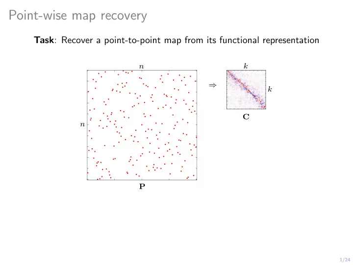
Point-wise map recovery

Task: Recover a point-to-point map from its functional representation

n n k k C P ⇒

1/24

Point-wise map recovery

Task: Recover a point-to-point map from its functional representation

n n k k rank(C) ≤ k ≪ n rank(P) ≤ n ⇒ ⇐

The inverse problem is highly underdetermined

1/24

Point-wise map recovery

Task: Recover a point-to-point map from its functional representation

n n k k rank(C) ≤ k ≪ n rank(P) ≤ n ⇒ ⇐

The inverse problem is highly underdetermined Need to use priors on the expected structure of the underlying map (e.g. bijectivity, smoothness, partiality, etc.)

2/24

Mapping delta functions

Algorithm: For each x ∈ M construct the delta function δx : M → R

x ∈ M

2/24

Mapping delta functions

Algorithm: For each x ∈ M construct the delta function δx : M → R

δx : M → R

2/24

Mapping delta functions

Algorithm: For each x ∈ M construct the delta function δx : M → R Compute its image δx → Tδx

δx : M → R Tδx : N → R

2/24

Mapping delta functions

Algorithm: For each x ∈ M construct the delta function δx : M → R Compute its image δx → Tδx Find argmaxy∈N Tδx(y)

δx : M → R Tδx : N → R

2/24

Mapping delta functions

Algorithm: For each x ∈ M construct the delta function δx : M → R Compute its image δx → Tδx Find argmaxy∈N Tδx(y) Doing this for all points is costly The maximum is delocalized due to the band-limited approximation of T!

δx : M → R Tδx : N → R

3/24

Linear assignment problem

For orthogonal bases ΦM, ΦN we can write C = Φ⊤

N PΦM

If the underlying map is known to be bijective, solve the LAP: min

Π∈{0,1}n×n −Π, ΦN CΦ⊤ M

s.t. Π⊤1 = 1 , Π1 = 1

Rodol` a et al. 2015

3/24

Linear assignment problem

For orthogonal bases ΦM, ΦN we can write C = Φ⊤

N PΦM

If the underlying map is known to be bijective, solve the LAP: min

Π∈{0,1}n×n CΦ⊤ M − Φ⊤ N Π2 F

s.t. Π⊤1 = 1 , Π1 = 1

Rodol` a et al. 2015

3/24

Linear assignment problem

For orthogonal bases ΦM, ΦN we can write C = Φ⊤

N PΦM

If the underlying map is known to be bijective, solve the LAP: min

Π∈{0,1}n×n CΦ⊤ M − Φ⊤ N Π2 F

s.t. Π⊤1 = 1 , Π1 = 1 The delta function δx has coefficients ai = φM

i (x) (a column of Φ⊤ M)

⇒ the image of all delta functions on M is simply CΦ⊤

M

Rodol` a et al. 2015; Ovsjanikov et al. 2012

3/24

Linear assignment problem

For orthogonal bases ΦM, ΦN we can write C = Φ⊤

N PΦM

If the underlying map is known to be bijective, solve the LAP: min

Π∈{0,1}n×n CΦ⊤ M − Φ⊤ N Π2 F

s.t. Π⊤1 = 1 , Π1 = 1 The delta function δx has coefficients ai = φM

i (x) (a column of Φ⊤ M)

⇒ the image of all delta functions on M is simply CΦ⊤

M

Interpretation: Seek the permutation aligning the k-dimensional spectral embeddings CΦ⊤

M and Φ⊤ M in the ℓ2 sense

Rodol` a et al. 2015; Ovsjanikov et al. 2012

3/24

Linear assignment problem

For orthogonal bases ΦM, ΦN we can write C = Φ⊤

N PΦM

If the underlying map is known to be bijective, solve the LAP: min

Π∈{0,1}n×n CΦ⊤ M − Φ⊤ N Π2 F

s.t. Π⊤1 = 1 , Π1 = 1 The delta function δx has coefficients ai = φM

i (x) (a column of Φ⊤ M)

⇒ the image of all delta functions on M is simply CΦ⊤

M

Interpretation: Seek the permutation aligning the k-dimensional spectral embeddings CΦ⊤

M and Φ⊤ M in the ℓ2 sense

Inefficient for large shapes

Rodol` a et al. 2015; Ovsjanikov et al. 2012

3/24

Linear assignment problem

For orthogonal bases ΦM, ΦN we can write C = Φ⊤

N PΦM

If the underlying map is known to be bijective, solve the LAP: min

Π∈{0,1}n×n CΦ⊤ M − Φ⊤ N Π2 F

s.t. Π⊤1 = 1 , Π1 = 1 The delta function δx has coefficients ai = φM

i (x) (a column of Φ⊤ M)

⇒ the image of all delta functions on M is simply CΦ⊤

M

Interpretation: Seek the permutation aligning the k-dimensional spectral embeddings CΦ⊤

M and Φ⊤ M in the ℓ2 sense

Inefficient for large shapes Lack of desirable properties on the recovered map (e.g. smoothness)

Rodol` a et al. 2015; Ovsjanikov et al. 2012

4/24

Nearest neighbors

Relaxing bijectivity to stochasticity constraints: min

P∈{0,1}n×m CΦ⊤ M − Φ⊤ N P2 F

s.t. P⊤1 = 1

Rodol` a et al. 2015

4/24

Nearest neighbors

Relaxing bijectivity to stochasticity constraints: min

P∈{0,1}n×m CΦ⊤ M − Φ⊤ N P2 F

s.t. P⊤1 = 1 Can be solved efficiently by a nearest-neighbor search in Rk

CΦ⊤

M

Φ⊤

N

Rodol` a et al. 2015; Ovsjanikov et al. 2012

5/24

Orthogonal refinement (ICP)

Orthogonal C ⇔ Area-preserving map Idea: Treat C as a pre-alignment, do orthogonal refinement to improve map quality

Ovsjanikov et al. 2012

5/24

Orthogonal refinement (ICP)

Orthogonal C ⇔ Area-preserving map Idea: Treat C as a pre-alignment, do orthogonal refinement to improve map quality Algorithm (ICP): P-step (nearest neighbors): P∗ = arg min

P∈{0,1}n×m C∗Φ⊤ M − Φ⊤ N P2 F

s.t. P⊤1 = 1

Ovsjanikov et al. 2012

5/24

Orthogonal refinement (ICP)

Orthogonal C ⇔ Area-preserving map Idea: Treat C as a pre-alignment, do orthogonal refinement to improve map quality Algorithm (ICP): P-step (nearest neighbors): P∗ = arg min

P∈{0,1}n×m C∗Φ⊤ M − Φ⊤ N P2 F

s.t. P⊤1 = 1 C-step (orthogonal Procrustes): C∗ = arg min

C∈Rk×k CΦ⊤ M − Φ⊤ N P∗2 F

s.t. C⊤C = I

Ovsjanikov et al. 2012

6/24

Non-orthogonal refinement (CPD)

For more general deformations (e.g. non-area preserving, non-isometric), do non-rigid refinement: min

P∈{0,1}n×m

DKL(CΦ⊤

M, Φ⊤ N P) + λ CΦ⊤ M − Φ⊤ N P2 Ω

s.t. P⊤1 = 1

Rodol` a et al. 2015

6/24

Non-orthogonal refinement (CPD)

For more general deformations (e.g. non-area preserving, non-isometric), do non-rigid refinement: min

P∈{0,1}n×m

DKL(CΦ⊤

M, Φ⊤ N P)

• Kullback−Leibler

+ λ CΦ⊤

M − Φ⊤ N P2 Ω

• coherence

s.t. P⊤1 = 1

Rodol` a et al. 2015

6/24

Non-orthogonal refinement (CPD)

For more general deformations (e.g. non-area preserving, non-isometric), do non-rigid refinement: min

P∈{0,1}n×m

DKL(CΦ⊤

M, Φ⊤ N P)

• Kullback−Leibler

+ λ CΦ⊤

M − Φ⊤ N P2 Ω

• coherence

s.t. P⊤1 = 1 · 2

Ω promotes smooth displacements

Rodol` a et al. 2015

6/24

Non-orthogonal refinement (CPD)

For more general deformations (e.g. non-area preserving, non-isometric), do non-rigid refinement: min

P∈{0,1}n×m

DKL(CΦ⊤

M, Φ⊤ N P)

• Kullback−Leibler

+ λ CΦ⊤

M − Φ⊤ N P2 Ω

• coherence

s.t. P⊤1 = 1 · 2

Ω promotes smooth displacements

λ controls the regularity (rigid for λ → ∞)

Rodol` a et al. 2015

6/24

Non-orthogonal refinement (CPD)

For more general deformations (e.g. non-area preserving, non-isometric), do non-rigid refinement: min

P∈{0,1}n×m

DKL(CΦ⊤

M, Φ⊤ N P)

• Kullback−Leibler

+ λ CΦ⊤

M − Φ⊤ N P2 Ω

• coherence

s.t. P⊤1 = 1 · 2

Ω promotes smooth displacements

λ controls the regularity (rigid for λ → ∞) Solved by coherent point drift

Rodol` a et al. 2015; Myronenko and Song 2010

6/24

Non-orthogonal refinement (CPD)

For more general deformations (e.g. non-area preserving, non-isometric), do non-rigid refinement: min

P∈{0,1}n×m

DKL(CΦ⊤

M, Φ⊤ N P)

• Kullback−Leibler

+ λ CΦ⊤

M − Φ⊤ N P2 Ω

• coherence

s.t. P⊤1 = 1 · 2

Ω promotes smooth displacements

λ controls the regularity (rigid for λ → ∞) Solved by coherent point drift Does not scale well

Rodol` a et al. 2015; Myronenko and Song 2010

7/24

Comparison

Reference Nearest neighbors Ovsjanikov et al. 2012; Rodol` a et al. 2015

7/24

Comparison

Reference Nearest neighbors ICP Ovsjanikov et al. 2012; Rodol` a et al. 2015

7/24

Comparison

Reference Nearest neighbors ICP CPD Ovsjanikov et al. 2012; Rodol` a et al. 2015

8/24

Product manifold filter (PMF)

Given P0 point-to-point (e.g. from nearest-neighbors), consider the LAP: max

Π∈{0,1}n×n trace(Π⊤KMP0K⊤ N )

s.t. Π⊤1 = 1 , Π1 = 1 with KM = exp(−D2

M/σ2) and KN = exp(−D2 N /σ2)

Vestner, Rodol` a, Litman, Bronstein, Cremers 2016

8/24

Product manifold filter (PMF)

Given P0 point-to-point (e.g. from nearest-neighbors), consider the LAP: max

Π∈{0,1}n×n trace(Π⊤KMP0K⊤ N )

s.t. Π⊤1 = 1 , Π1 = 1 with KM = exp(−D2

M/σ2) and KN = exp(−D2 N /σ2)

Interpretation as an inference problem from stochastic data

Vestner, Rodol` a, Litman, Bronstein, Cremers 2016

8/24

Product manifold filter (PMF)

Given P0 point-to-point (e.g. from nearest-neighbors), consider the LAP: max

Π∈{0,1}n×n trace(Π⊤KMP0K⊤ N )

s.t. Π⊤1 = 1 , Π1 = 1 with KM = exp(−D2

M/σ2) and KN = exp(−D2 N /σ2)

Interpretation as an inference problem from stochastic data The similarity induces smooth maps

Vestner, Rodol` a, Litman, Bronstein, Cremers 2016

8/24

Product manifold filter (PMF)

Given P0 point-to-point (e.g. from nearest-neighbors), consider the LAP: max

Π∈{0,1}n×n trace(Π⊤KMP0K⊤ N )

s.t. Π⊤1 = 1 , Π1 = 1 with KM = exp(−D2

M/σ2) and KN = exp(−D2 N /σ2)

Auction algorithm: O(n2 log n) average complexity

Vestner, Rodol` a, Litman, Bronstein, Cremers 2016; Bertsekas 1998

8/24

Product manifold filter (PMF)

Given P0 point-to-point (e.g. from nearest-neighbors), consider the LAP: max

Π∈{0,1}n×n trace(Π⊤KMP0K⊤ N )

s.t. Π⊤1 = 1 , Π1 = 1 with KM = exp(−D2

M/σ2) and KN = exp(−D2 N /σ2)

Auction algorithm: O(n2 log n) average complexity Multi-scale acceleration reduces complexity by orders of magnitude

Vestner, Rodol` a, Litman, Bronstein, Cremers 2016; Bertsekas 1998

8/24

Product manifold filter (PMF)

Given P0 point-to-point (e.g. from nearest-neighbors), consider the LAP: max

Π∈{0,1}n×n trace(Π⊤KMP0K⊤ N )

s.t. Π⊤1 = 1 , Π1 = 1 with KM = exp(−D2

M/σ2) and KN = exp(−D2 N /σ2)

Auction algorithm: O(n2 log n) average complexity Multi-scale acceleration reduces complexity by orders of magnitude

Vestner, Rodol` a, Litman, Bronstein, Cremers 2016; Bertsekas 1998

8/24

Product manifold filter (PMF)

Given P0 point-to-point (e.g. from nearest-neighbors), consider the LAP: max

Π∈{0,1}n×n trace(Π⊤KMP0K⊤ N )

s.t. Π⊤1 = 1 , Π1 = 1 with KM = exp(−D2

M/σ2) and KN = exp(−D2 N /σ2)

Auction algorithm: O(n2 log n) average complexity Multi-scale acceleration reduces complexity by orders of magnitude

Vestner, Rodol` a, Litman, Bronstein, Cremers 2016; Bertsekas 1998

9/24

Examples

1% 3% 5% 7% ×diam

ICP CPD

Vestner, Rodol` a, Litman, Bronstein, Cremers 2016

9/24

Examples

1% 3% 5% 7% ×diam

ICP CPD ICP+PMF CPD+PMF

Vestner, Rodol` a, Litman, Bronstein, Cremers 2016

10/24

Comparison

50 60 70 80 90 100

% correspondences

2 4 6 8 10

Geodesic error (in % of the diameter)

NN Bijective NN NN+PMF

• Bij. NN+PMF

CPD CPD+PMF

Vestner, Rodol` a, Litman, Bronstein, Cremers 2016

11/24

Application: Point-to-point map improvement

Refinement can be used to improve noisy maps obtained with any point-wise matching pipeline

reference input improved Kim et al. 2011; Ovsjanikov et al. 2012

12/24

Application: Segmentation transfer

Transfer indicator functions for each segment, without resorting to a point-to-point correspondence

input segment image transfer Ovsjanikov et al. 2012

13/24

Application: Simultaneous shape editing

Coupled bases allow to solve for the deformation field in the functional domain, and transfer pose to multiple shapes simultaneously

Kovnatsky, Bronstein, Bronstein, Glashoff, Kimmel 2013; Rong et al. 2008

14/24

Application: Partial scanning

Litany, Rodol` a, Bronstein, Bronstein, Cremers 2016

14/24

Application: Partial scanning

Litany, Rodol` a, Bronstein, Bronstein, Cremers 2016

14/24

Application: Partial scanning

Litany, Rodol` a, Bronstein, Bronstein, Cremers 2016

14/24

Application: Partial scanning

Litany, Rodol` a, Bronstein, Bronstein, Cremers 2016

14/24

Application: Partial scanning

Litany, Rodol` a, Bronstein, Bronstein, Cremers 2016

15/24

Application: Shape retrieval

The average ratio of the norms of the diagonal and off-diagonal elements

• f C can be used as a global similarity criterion

Kovnatsky, Bronstein, Bronstein, Glashoff, Kimmel 2013

16/24

Application: Object detection and recognition

The final energy can be used as an indicator that the object is present in the scene; localization does not require a point-wise correspondence

query retrieved object query retrieved object Cosmo, Rodol` a, Masci, Torsello, Bronstein 2016

17/24

Application: Improving map collections

The pairwise maps can be improved by considering the context

Nguyen et al. 2011; Ovsjanikov, Ben-Chen, Solomon, Butscher, Guibas 2012; Kovnatsky, Glashoff, Bronstein 2016

17/24

Application: Improving map collections

The pairwise maps can be improved by considering the context Compose maps along cycles mX,Y = mZ,Y ◦ mX,Z = CZ,Y CX,Z

Nguyen et al. 2011; Ovsjanikov, Ben-Chen, Solomon, Butscher, Guibas 2012; Kovnatsky, Glashoff, Bronstein 2016

17/24

Application: Improving map collections

The pairwise maps can be improved by considering the context Compose maps along cycles mX,Y = mZ,Y ◦ mX,Z = CZ,Y CX,Z Compare to the identity C − IF

Nguyen et al. 2011; Ovsjanikov, Ben-Chen, Solomon, Butscher, Guibas 2012; Kovnatsky, Glashoff, Bronstein 2016

17/24

Application: Improving map collections

The pairwise maps can be improved by considering the context Compose maps along cycles mX,Y = mZ,Y ◦ mX,Z = CZ,Y CX,Z Compare to the identity C − IF Replace faulty maps with composites along shortest paths

Nguyen et al. 2011; Ovsjanikov, Ben-Chen, Solomon, Butscher, Guibas 2012; Kovnatsky, Glashoff, Bronstein 2016

17/24

Application: Improving map collections

The pairwise maps can be improved by considering the context Compose maps along cycles mX,Y = mZ,Y ◦ mX,Z = CZ,Y CX,Z Compare to the identity C − IF Replace faulty maps with composites along shortest paths Optimize over cycle-consistent functional maps minC C∗ + λ

(i,j)∈G CijAij − Bij2,1

Nguyen et al. 2011; Ovsjanikov, Ben-Chen, Solomon, Butscher, Guibas 2012; Kovnatsky, Glashoff, Bronstein 2016; Huang, Wang, Guibas 2014

18/24

Application: Analysis of shape collections

Find structural similarities in heterogeneous shape collections

consistent basis functions ⇒ Huang, Wang, Guibas 2014

18/24

Application: Analysis of shape collections

Find structural similarities in heterogeneous shape collections

co-segmentation ⇒ Huang, Wang, Guibas 2014

18/24

Application: Analysis of shape collections

With shape differences we can compare shapes as well as deformations, and therefore find similar shapes

query ROI 1 2 3 4 query ROI 1 2 3 4 Huang, Wang, Guibas 2014

18/24

Application: Analysis of shape collections

With shape differences we can compare shapes as well as deformations, and therefore find similar shapes find similar deformations

Huang, Wang, Guibas 2014; Rustamov, Ovsjanikov, Azencot, Ben-Chen, Chazal, Guibas 2013

18/24

Application: Analysis of shape collections

With shape differences we can compare shapes as well as deformations, and therefore find similar shapes find similar deformations

Huang, Wang, Guibas 2014; Rustamov, Ovsjanikov, Azencot, Ben-Chen, Chazal, Guibas 2013

18/24

Application: Analysis of shape collections

With shape differences we can compare shapes as well as deformations, and therefore find similar shapes find similar deformations / synthesize new deformations

Huang, Wang, Guibas 2014; Rustamov, Ovsjanikov, Azencot, Ben-Chen, Chazal, Guibas 2013; Boscaini, Eynard, Kourounis, Bronstein 2015

18/24

Application: Analysis of shape collections

With shape differences we can compare shapes as well as deformations, and therefore find similar shapes find similar deformations / synthesize new deformations

Huang, Wang, Guibas 2014; Rustamov, Ovsjanikov, Azencot, Ben-Chen, Chazal, Guibas 2013; Boscaini, Eynard, Kourounis, Bronstein 2015

19/24

Application: Shape exploration

Using shape differences we can interpolate/extrapolate the difference between corresponding regions of a shape pair

source target interpolate extrapolate Huang, Wang, Guibas 2014

19/24

Application: Shape exploration

Using shape differences we can interpolate/extrapolate the difference between corresponding regions of a shape pair

source interpolated target Huang, Wang, Guibas 2014; Rustamov, Ovsjanikov, Azencot, Ben-Chen, Chazal, Guibas 2013

20/24

Application: Shape interpolation

Linear interpolation in shape differences space: Dα = (1 − α)I + αD α = 1

20/24

Application: Shape interpolation

Linear interpolation in shape differences space: Dα = (1 − α)I + αD α = 1 α = 0 α = . 5 α = 1 . 5

21/24

Application: Image co-segmentation

Network of maps can be used for co-segmentation of images

consistent functional maps segmentations Wang, Huang, Guibas 2013; Wang, Huang, Ovsjanikov, Guibas 2014

21/24

Application: Image co-segmentation

Network of maps can be used for co-segmentation of images

Wang, Huang, Guibas 2013; Wang, Huang, Ovsjanikov, Guibas 2014

22/24

Things we did not cover

Point-wise map recovery by vector field flow Point-wise map recovery for partial functional maps Functional fluids Visualization and analysis of functional maps Matching via quotient spaces Permuted sparse coding Functional correspondence via matrix completion Coupled functional maps Functional maps for image data . . .

Corman et al. 2015; Rodol` a et al. 2016; Azencot et al. 2015; Vantzos et al. 2016; Ovsjanikov et al. 2013; Pokrass et al. 2013; Kovnatsky et al. 2015; Eynard et al. 2016; Wang et al. 2013

23/24

Summary

Considering mappings through their action on functions is simpler and more flexible

23/24

Summary

Considering mappings through their action on functions is simpler and more flexible The size of these objects can be controlled in the discrete setting

23/24

Summary

Considering mappings through their action on functions is simpler and more flexible The size of these objects can be controlled in the discrete setting Shape differences provide a way to compare shapes and deformations in an informative way

23/24

Summary

Considering mappings through their action on functions is simpler and more flexible The size of these objects can be controlled in the discrete setting Shape differences provide a way to compare shapes and deformations in an informative way Functional maps provide a common language in which many problems in geometry and data processing can be expressed

23/24

Summary

Considering mappings through their action on functions is simpler and more flexible The size of these objects can be controlled in the discrete setting Shape differences provide a way to compare shapes and deformations in an informative way Functional maps provide a common language in which many problems in geometry and data processing can be expressed Very easy to pick up!

23/24

Summary

Considering mappings through their action on functions is simpler and more flexible The size of these objects can be controlled in the discrete setting Shape differences provide a way to compare shapes and deformations in an informative way Functional maps provide a common language in which many problems in geometry and data processing can be expressed Very easy to pick up! Code and course notes available at: http://www.lix.polytechnique.fr/~maks/fmaps_course/

24/24

Thank you!