Todays Topic CSE-571 EKF Feature-Based SLAM Probabilistic Robotics - PDF document

10/27/15 Today’s Topic CSE-571 ¨ EKF Feature-Based SLAM Probabilistic Robotics ¤ State Representation ¤ Process / Observation Models ¤ Landmark Initialization ¤ Robot-Landmark Correlation SLAM: Simultaneous Localization and Mapping Many slides courtesy of Ryan Eustice, Cyrill Stachniss, John Leonard The SLAM Problem SLAM Applications 3 A robot is exploring an 4 Indoors Undersea unknown, static environment. 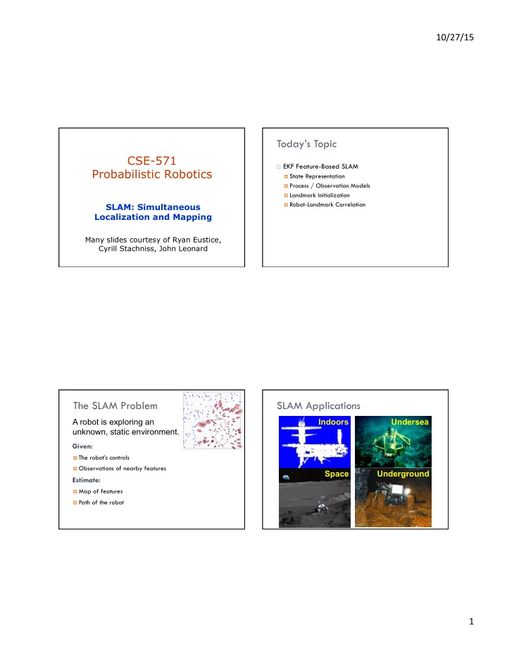Given: ¤ The robot’s controls ¤ Observations of nearby features Space Underground Estimate: ¤ Map of features ¤ Path of the robot 1

10/27/15 Illustration of SLAM Illustration of SLAM without Landmarks without Landmarks With only dead reckoning, vehicle With only dead reckoning, vehicle pose uncertainty grows without pose uncertainty grows without bound bound Courtesy J. Leonard Courtesy J. Leonard Illustration of SLAM Illustration of SLAM without Landmarks without Landmarks With only dead reckoning, vehicle With only dead reckoning, vehicle pose uncertainty grows without pose uncertainty grows without bound bound Courtesy J. Leonard Courtesy J. Leonard 2

10/27/15 Illustration of SLAM Illustration of SLAM without Landmarks without Landmarks With only dead reckoning, vehicle With only dead reckoning, vehicle pose uncertainty grows without pose uncertainty grows without bound bound Courtesy J. Leonard Courtesy J. Leonard Repeat, with Measurements of Mapping with Raw Odometry Landmarks ¨ First position: two features observed Courtesy J. Leonard 3

10/27/15 Illustration of SLAM with Landmarks Illustration of SLAM with Landmarks ¨ Second position: two new features ¨ Re-observation of first two features observed results in improved estimates for both vehicle and feature Courtesy J. Leonard Courtesy J. Leonard Illustration of SLAM with Landmarks Illustration of SLAM with Landmarks ¨ Third position: two additional ¨ Re-observation of first four features results in improved location estimates features added to map for vehicle and all features Courtesy J. Leonard Courtesy J. Leonard 4

10/27/15 SLAM Using Landmarks Illustration of SLAM with Landmarks MIT Indoor Track ¨ Process continues as the vehicle moves through the environment Courtesy J. Leonard Courtesy J. Leonard Test Environment (Point Landmarks) View from Vehicle Courtesy J. Leonard Courtesy J. Leonard 5

10/27/15 SLAM Using Landmarks Comparison with Ground Truth 1. Move 2. Sense 3. Associate measurements with known features 4. Update state estimates for robot and previously mapped features 5. Find new features from unassociated measurements 6. Initialize new features 7. Repeat odometry MIT Indoor Track SLAM result Courtesy J. Leonard Simultaneous Localization and Definition of the SLAM Problem Mapping (SLAM) ¨ Building a map and locating the robot in the map at Given the same time ¤ The robot ’ s controls ¨ Chicken-and-egg problem ¤ Observations map Wanted ¤ Map of the environment ¤ Path of the robot localize Courtesy: Cyrill Stachniss Courtesy: Cyrill Stachniss 6

10/27/15 Three Main Paradigms Bayes Filter ¨ Recursive filter with prediction and correction step Kalman Particle Graph- ¨ Prediction filter filter based ¨ Correction Courtesy: Cyrill Stachniss Courtesy: Cyrill Stachniss EKF for Online SLAM Extended Kalman Filter Algorithm ¨ We consider here the Kalman filter as a solution to the online SLAM problem Courtesy: Thrun, Burgard, Fox Courtesy: Cyrill Stachniss 7

10/27/15 EKF SLAM EKF SLAM: State Representation ¨ Application of the EKF to SLAM ¨ Map with n landmarks: (3+2n)-dimensional Gaussian ¨ Estimate robot’s pose and locations of landmarks in the environment ¨ Belief is represented by ¨ Assumption: known correspondences ¨ State space (for the 2D plane) is Courtesy: Cyrill Stachniss Courtesy: Cyrill Stachniss EKF SLAM: State Representation EKF SLAM: State Representation ¨ More compactly ¨ Even more compactly (note: ) Courtesy: Cyrill Stachniss Courtesy: Cyrill Stachniss 8

10/27/15 EKF SLAM: Filter Cycle EKF SLAM: State Prediction 1. State prediction 2. Measurement prediction 3. Measurement 4. Data association 5. Update Courtesy: Cyrill Stachniss Courtesy: Cyrill Stachniss EKF SLAM: Obtained EKF SLAM: Measurement Measurement Prediction Courtesy: Cyrill Stachniss Courtesy: Cyrill Stachniss 9

10/27/15 EKF SLAM: Data Association and EKF SLAM: Update Step Difference Between h(x) and z Courtesy: Cyrill Stachniss Courtesy: Cyrill Stachniss EKF SLAM: Concrete Example Initialization Setup ¨ Robot starts in its own reference frame (all landmarks unknown) ¨ Robot moves in the 2D plane ¨ 2N+3 dimensions ¨ Velocity-based motion model ¨ Robot observes point landmarks ¨ Range-bearing sensor ¨ Known data association ¨ Known number of landmarks Courtesy: Cyrill Stachniss Courtesy: Cyrill Stachniss 10

10/27/15 Prediction Step (Motion) Extended Kalman Filter Algorithm ¨ Goal: Update state space based on the robot’s motion ¨ Robot motion in the plane ¨ How to map that to the 2N+3 dim space? Courtesy: Cyrill Stachniss Courtesy: Cyrill Stachniss Update the State Space Extended Kalman Filter Algorithm ¨ From the motion in the plane DONE ¨ to the 2N+3 dimensional space Courtesy: Cyrill Stachniss Courtesy: Cyrill Stachniss 11

10/27/15 Update Covariance This Leads to the Time Propagation ¨ The function only affects the robot’s motion and not the landmarks Apply & DONE Jacobian of the motion (3x3) Identity (2N x 2N) Courtesy: Cyrill Stachniss Courtesy: Cyrill Stachniss EKF SLAM: Correction Step Extended Kalman Filter Algorithm ¨ Known data association ¨ : i -th measurement at time t observes the landmark with index j DONE ¨ Initialize landmark if unobserved DONE ¨ Compute the expected observation ¨ Compute the Jacobian of ¨ Proceed with computing the Kalman gain Courtesy: Cyrill Stachniss Courtesy: Cyrill Stachniss 12

10/27/15 Range-Bearing Observation Jacobian for the Observation ¨ Range-Bearing observation ¨ Based on ¨ If landmark has not been observed observed estimated ¨ Compute the Jacobian relative measurement location of robot’s landmark j location Courtesy: Cyrill Stachniss Courtesy: Cyrill Stachniss Jacobian for the Observation Next Steps as Specified… ¨ Use the computed Jacobian DONE DONE ¨ map it to the high dimensional space Courtesy: Cyrill Stachniss Courtesy: Cyrill Stachniss 13

10/27/15 EKF SLAM – Correction (1/2) Extended Kalman Filter Algorithm DONE DONE Apply & DONE Apply & DONE Apply & DONE Courtesy: Cyrill Stachniss Courtesy: Cyrill Stachniss EKF SLAM – Correction (2/2) EKF SLAM Complexity ¨ Cubic complexity depends only on the measurement dimensionality ¨ Cost per step: dominated by the number of landmarks: ¨ Memory consumption: ¨ The EKF becomes computationally intractable for large maps! Courtesy: Cyrill Stachniss Courtesy: Cyrill Stachniss 14

10/27/15 EKF SLAM Correlations EKF SLAM Correlations 72 ¨ In the limit, the landmark estimates become fully correlated Blue path = true path Red path = estimated path Black path = odometry ¨ Approximate the SLAM posterior with a high-dimensional Gaussian [Smith & Cheesman, 1986] … ¨ Single hypothesis data association Courtesy: Dissanayake Courtesy: M. Montemerlo EKF SLAM Correlations EKF SLAM Correlations Map Correlation matrix Map Correlation matrix Courtesy: M. Montemerlo Courtesy: M. Montemerlo 15

10/27/15 EKF SLAM Uncertainties EKF SLAM Correlations ¨ The determinant of any sub-matrix of the map covariance matrix decreases monotonically ¨ New landmarks are initialized with maximum uncertainty Map Correlation matrix Courtesy: Dissanayake Courtesy: M. Montemerlo Data Association in SLAM Data Association ¨ Given an environment map 77 ¨ And a set of sensor observations ¨ Associate observations with map elements Robot pose uncertainty ¨ In the real world, the mapping between observations and landmarks is unknown ¨ Picking wrong data associations can have catastrophic consequences ¤ EKF SLAM is brittle in this regard Vision Laser ¨ Pose error correlates data associations 16

10/27/15 Difficulties: clutter Difficulties: clutter ¨ Influence of the type, density, precision and 10000 ¨ Vertical Edge Monocular vision: robustness of features considered: 8000 10000 6000 8000 4000 Laser scanner: 6000 2000 • Small amount of 4000 0 features (n ) 2000 • Small amount of -2000 -6000 -4000 -2000 0 2000 4000 6000 measurements (m ) 0 ¨ Many features (n large) • Low spuriousness -2000 High clutter ¨ Many measurements (m large) -6000 -4000 -2000 0 2000 4000 6000 ¨ no depth information Low clutter ¨ higher spuriousness Difficulties: imprecision Loop-Closing ¨ Both the sensor and the vehicle introduce imprecision 10000 10000 ¨ Loop-closing means recognizing an already mapped area 8000 8000 ¨ Data association under 6000 6000 ¤ high ambiguity 4000 4000 ¤ possible environment symmetries 2000 2000 ¨ Uncertainties collapse after a loop-closure (whether 0 0 the closure was correct or not) -2000 -2000 -6000 -4000 -2000 0 2000 4000 6000 -6000 -4000 -2000 0 2000 4000 6000 Vertical Edge Trinocular Robot imprecision: vision: introduces CORRELATED error variable depth precision good angular precision Courtesy: Cyrill Stachniss 17

10/27/15 Before the Loop-Closure After the Loop-Closure Courtesy: K. Arras Courtesy: K. Arras Example: Victoria Park Dataset Victoria Park: Data Acquisition Courtesy: E. Nebot Courtesy: E. Nebot 18