Self-calibration and unordered SfM 3D photography course schedule - PowerPoint PPT Presentation

Self-calibration and unordered SfM

3D photography course schedule Topic Feb 21 Introduction Feb 28 Lecture: Geometry, Camera Model, Calibration Mar 7 Lecture: Features & Correspondences Mar 14 Project Proposals Mar 21 Lecture: Epipolar Geometry Mar 28 Depth Estimation + 2 papers Apr 4 Single View Geometry + 2 papers Apr 11 Active Ranging and Structured Light + 2 papers Apr 18 Project Updates Apr. 25 --- Easter --- May 2 SLAM + 2 papers May 9 3D & Registration + 2 papers May 16 SfM/Self Calibration + 2 papers May 23 Shape from Silhouettes + 2 papers May 30 Final Projects

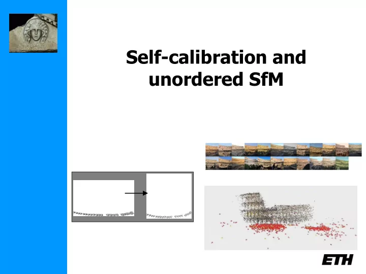
Evaluation • Today: May, 16 th , 2011 • Course ID: 252-0579-00G

Unordered/Uncalibrated Structure from Motion Scenarios: • “folders” with pictures, photo collections • Unknown cameras/photos Similar “multiple view geometry” as SLAM, but Challenges: • Finding Corresponding Images/Features • Self-Calibration

Simpler Case: Unord./Uncalib. Panorama ( Brown/Lowe, ICCV’03, IJCV’07 ) • Folder with photos from same position • Estimate orientation, focal length for each image (assume defaults for other params) • Stitch images

Simpler Case: Unord./Uncalib. Panorama ( Brown/Lowe, ICCV’03, IJCV’07 ) • SIFT features -> kd-tree • Find nearest neighbors in descriptor space • Pick image pair with highest #matches • Robust estimation of homography (R,f 1 ,f 2 ) • (Bundle Adjustment)

Unordered SfM (Schaffalitzky/Zisserman ECCV02) (Brown/Lowe 3DIM05) (Snavely et al. SIGGRAPH06) • Finding Corresponding Images/Features similar as in pano • Self-Calibration often simplified model K=diag(f,f,1) - initial f from pairs, - optimize in bundle adjustment -> presented afterwards !

Building Rome on a cloudless day (Frahm et al. ECCV10) • GIST & clustering (1h35) Dense Reconstruction (1h58) SIFT & Geometric verification (11h36) Some numbers 1PC • 2.88M images • SfM & Bundle (8h35) 100k clusters • 22k SfM with 307k images • 63k 3D models • Largest model 5700 images • Total time 23h53 •

Self-calibration • Self-calibration • Dual Absolute Quadric • Critical Motion Sequences

Motivation • Avoid explicit calibration procedure • Complex procedure • Need for calibration object • Need to maintain calibration

Motivation • Allow flexible acquisition • No prior calibration necessary • Possibility to vary intrinsics • Use archive footage

Projective ambiguity Reconstruction from uncalibrated images  projective ambiguity on reconstruction    1  m P M ( PT )( T M) P ´M´

Stratification of geometry Projective Affine Metric 7 DOF 12 DOF 15 DOF absolute conic plane at infinity parallelism angles, rel.dist. More general More structure

Constraints ? Scene constraints • Parallellism, vanishing points, horizon, ... • Distances, positions, angles, ... Unknown scene  no constraints Camera extrinsics constraints – Pose, orientation, ... Unknown camera motion  no constraints Camera intrinsics constraints – Focal length, principal point, aspect ratio & skew Perspective camera model too general  some constraints

Euclidean projection matrix Factorization of Euclidean projection matrix     T T P K R R t   f s u x x    K f u Intrinsics: (camera geometry)   y y   1   Extrinsics:   R , t (camera motion) Note: every projection matrix can be factorized, but only meaningful for euclidean projection matrices

Constraints on intrinsic parameters   f s u x x    K f u   y y   1   Constant   K K e.g. fixed camera:  1 2 Known  e.g. rectangular pixels: s 0   square pixels: f f , s 0 x y     w h  principal point known: u , u  ,  x y 2 2  

Self-calibration Upgrade from projective structure to metric structure using constraints on intrinsic camera parameters • Constant intrinsics (Faugeras et al. ECCV´92, Hartley´93, Triggs´97, Pollefeys et al. PAMI´99, ...) • Some known intrinsics, others varying (Heyden&Astrom CVPR´97, Pollefeys et al. ICCV´98,...) • Constraints on intrinsics and restricted motion (e.g. pure translation, pure rotation, planar motion) (Moons et al.´94, Hartley ´94, Armstrong ECCV´96, ...)

A counting argument • To go from projective (15DOF) to metric (7DOF) at least 8 constraints are needed • Minimal sequence length should satisfy            m # known m 1 # fixed 8 • Independent of algorithm • Assumes general motion (i.e. not critical)

Outline • Introduction • Self-calibration • Dual Absolute Quadric • Critical Motion Sequences

The Dual Absolute Quadric   I 0    *   T 0 0   The absolute dual quadric Ω * ∞ is a fixed conic under the projective transformation H iff H is a similarity 1. 8 dof 2. plane at infinity π ∞ is the nullvector of Ω ∞  3. Angles: T * π π    cos 1 2    T  * T  * π π π π   1 1 2 2

Absolute Dual Quadric and Self-calibration Eliminate extrinsics from equation Equivalent to projection of Dual Abs.Quadric Dual Abs.Quadric also exists in projective world     T * T 1 * T T T KK P Ω P ( PT )( T Ω T )( T P )   * P  T P ´ Ω ´ ´    * * Ω ´ Ω Transforming world so that  reduces ambiguity to similarity

Absolute Dual Quadric and Self-calibration Projection equation:     T T ω P Ω P K K  * i i i i i Translate constraints on K  * through projection equation to constraints on  * Absolute conic = calibration object which is always present but can only be observed through constraints on the intrinsics

Constraints on  *       2 2 2 f s c sf c c c x x y x y x      * 2 2 ω sf c c f c c    y x y y y y   c c 1   x y #constraints condition constraint type Zero skew quadratic m  * * * * ω ω ω ω 12 33 13 23 Principal point   linear * * 2 m ω ω 0 13 23 Zero skew (& p.p.) linear m 12  ω * 0 Fixed aspect ratio quadratic m-1  * * * * ω ω' ω ω' (& p.p.& Skew) 11 22 22 11  Known aspect ratio * * linear ω ω m 11 22 (& p.p.& Skew)  * * ω ω Focal length linear m 33 11 (& p.p. & Skew)

Linear algorithm (Pollefeys et al.,ICCV´98/IJCV´99) Assume everything known, except focal length         T T P Ω P P Ω P 0 ˆ   2 f 0 0 11 22       T P Ω P 0 ˆ *  2   * T ω 0 f 0 P P 12       T P Ω P 0   0 0 1 13       T P Ω P 0 23 Yields 4 constraint per image Note that rank-3 constraint is not enforced

Linear algorithm revisited (Pollefeys et al., ECCV‘02) Weighted linear equations     1   ˆ     T T P Ω P P Ω P 0 2 f 0 0 11 22 0 . 2     1  ˆ  T P Ω P 0 T  2 KK 0 f 0   0 . 01 12   1     T P Ω P 0 0 0 1   0 11 . 13     T P Ω P 0 0 . 1 23     1   T  T  P Ω P P Ω P 0 11 33 9     1     T T P Ω P P Ω P 0 22 33 9 assumptions ˆ  0     c 0 . 1 s 0 log( f ) log( 1 ) log( 3 ) x ˆ f  0  c 0 . 1   log( ˆ ) log( 1 ) log( 1 . 1 ) x y f y

Projective to metric Compute T from   I 0 ~ ~ ~    * T - 1 - T * I T Ω T or T I T Ω with I     T 0 0   using eigenvalue decomposition of Ω *  and then obtain metric reconstruction as PT -1 and T M

Alternatives: (Dual) image of absolute conic • Equivalent to Absolute Dual Quadric   * * T ω P Ω P    * * T ω H ω H    • Practical when H  can be computed first • Pure rotation (Hartley’94, Agapito et al.’98,’99) • Vanishing points, pure translations, modulus constraint, …

Note that in the absence of skew the IAC can be more practical than the DIAC!    2 2 f c c c c x x x y x      * 2 2 T ω c c f c c KK    x y y y y   c c 1   x y    2 2 f 0 f c y y x   1     2 2 T 1 ω 0 f f c ( KK )    x x y 2 2 f f   x y     2 2 2 2 2 2 2 2 f c f c f f f c f c   y x x y x y y x x y

Kruppa equations         T T   * * T * T e' ω e' e' H ω H e' F ω F          Limit equations to epipolar geometry Only 2 independent equations per pair But independent of plane at infinity