
SLIDE 1
1
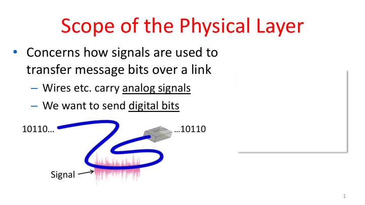
Scope of the Physical Layer
- Concerns how signals are used to
transfer message bits over a link
– Wires etc. carry analog signals – We want to send digital bits
…10110
10110… Signal
Scope of the Physical Layer Concerns how signals are used to - - PowerPoint PPT Presentation
Scope of the Physical Layer Concerns how signals are used to transfer message bits over a link Wires etc. carry analog signals We want to send digital bits 10110 10110 Signal 1 Simple Link Model Well end with an
1
…10110
10110… Signal
CSE 461 University of Washington 2
Delay D, Rate R Message
CSE 461 University of Washington 3
T-delay = M (bits) / Rate (bits/sec) = M/R seconds
P-delay = Length / speed of signals = Length / ⅔c = D seconds
CSE 461 University of Washington 4
CSE 461 University of Washington 5
– 1 Mbps = 1,000,000 bps, 1 KB = 210 bytes
Prefix Exp. prefix exp. K(ilo) 103 m(illi) 10-3 M(ega) 106 μ(micro) 10-6 G(iga) 109 n(ano) 10-9
CSE 461 University of Washington 6
D = 5 ms, R = 56 kbps, M = 1250 bytes L = 5 ms + (1250x8)/(56 x 103) sec = 184 ms!
D = 50 ms, R = 10 Mbps, M = 1250 bytes L = 50 ms + (1250x8) / (10 x 106) sec = 51 ms
– Often, one delay component dominates
CSE 461 University of Washington 7
CSE 461 University of Washington 8
110101000010111010101001011
weights of harmonic frequencies Signal over time
9
amplitude
Lost!
10
Lost! Lost! Bandwidth
11
CSE 461 University of Washington 12
13
14
15
16
WiFi WiFi
17
802.11 b/g/n 802.11a/g/n
18
…10110
10110…
19
1 1 1 1 1 1 1 +V
20
1 1 1 1 1 1 1 +V
21
NRZ signal of bits Amplitude shift keying Frequency shift keying Phase shift keying
22
23
24
25
Credit: Courtesy MIT Museum
Electromechanical mouse that “solves” mazes!
26
27
28
29
30
31
Upstream Downstream 26 – 138 kHz 0-4 kHz 143 kHz to 1.1 MHz Telephone Freq. Voice Up to 1 Mbps Up to 12 Mbps
CSE 461 University of Washington 32
Physical Link Network Transport Application
CSE 461 University of Washington 33
Frame
CSE 461 University of Washington 34
CSE 461 University of Washington 35
– Delimiting start/end of frames
– Handling errors
– Handling loss
– 802.11, classic Ethernet
– Modern Ethernet
CSE 461 University of Washington 36
…10110 … Um?
CSE 461 University of Washington 37
CSE 461 University of Washington 38
CSE 461 University of Washington 39
CSE 461 University of Washington 40
CSE 461 University of Washington 41
CSE 461 University of Washington 42
CSE 461 University of Washington 43
CSE 461 University of Washington 44
CSE 461 University of Washington 45
Transmitted bits with stuffing Data bits
CSE 461 University of Washington 46
Transmitted bits with stuffing Data bits