Sample Size Power, Sample Size, and the FDR How many observations - PDF document

Sample Size Power, Sample Size, and the FDR “How many observations do we need?” Depends on Peter Dalgaard • Design • Standard error of measurements Department of Biostatistics • Effect size University of Copenhagen • How sure you want to be of finding it Center for Bioinformatics, Univ.Copenhagen, June 2005 Reminders Variation of Observations and Means (Continuous data) One-sample (or paired, differences): dnorm(x, sd = sqrt(1/20)) � SEM = s × 1 / n 1.5 Significance if | ¯ x − µ 0 | 1.0 > t . 975 ( DF ) SEM 0.5 Two-sample: � SEDM = s × 1 / n 1 + 1 / n 2 0.0 | ¯ x 1 − ¯ x 2 | −3 −2 −1 0 1 2 3 SEDM > t . 975 ( DF ) x t . 975 ( DF ) ≈ 2. Notice that SE(D)M decreases with n . t Test Type I and Type II Errors 0.4 0.3 A test of a hypothesis can go wrong in two ways: dt(t, 38) Type I error: Rejecting a true null hypothesis 0.2 Type II error: Accepting a false null hypothesis 0.1 Error probabilities: α resp. β α : Significance level (0.05, e.g.) 0.0 1 − β : Power – probability of detecting difference −3 −2 −1 0 1 2 3 Notice that the power depends on the effect size as well as on t the number of observations and significance level. • If there is no (true) difference then there is little chance of getting an observation in the tails • If there is a difference, then the center of the distribution is shifted. 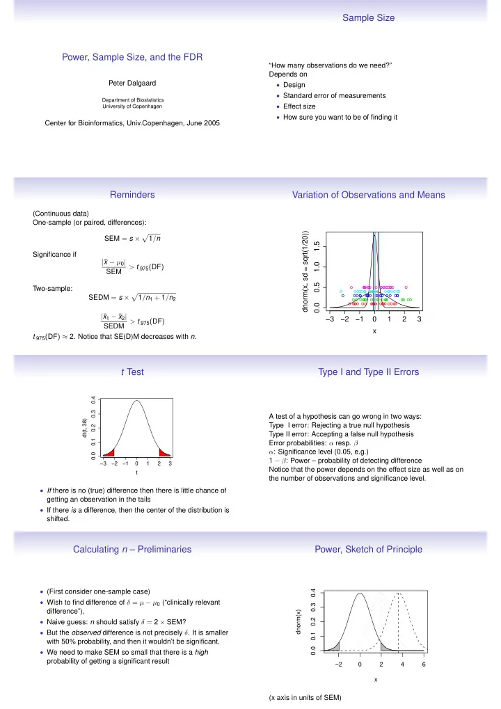Calculating n – Preliminaries Power, Sketch of Principle • (First consider one-sample case) 0.4 • Wish to find difference of δ = µ − µ 0 (“clinically relevant 0.3 difference”), dnorm(x) 0.2 • Naive guess: n should satisfy δ = 2 × SEM? • But the observed difference is not precisely δ . It is smaller 0.1 with 50% probability, and then it wouldn’t be significant. 0.0 • We need to make SEM so small that there is a high probability of getting a significant result −2 0 2 4 6 x (x axis in units of SEM)

Size of SEM relative to δ Calculating n (Notice: These formulas assume known SD. Watch out if n is very small. More accurate formulas in R’s power.t.test ) Just insert SEM = σ/ √ n in δ = 3 . 24 × SEM and solve for n : z p quantiles in normal distribution, z 0 . 975 = 1 . 96, etc. Two-tailed test, α = 0 . 05, power 1 − β = 0 . 90 n = ( 3 . 24 × σ/δ ) 2 δ = ( 1 . 96 + k ) × SEM (for two-sided test at level α = 0 . 05, with power 1 − β = 0 . 90) k is distance between middle and right peak in slide 8. Find k General formula for arbitrary α and β : so that there is a probability of 0.90 of observing a difference of at least 1 . 96 × SEM. n = (( z 1 − α/ 2 + z 1 − β ) × ( σ/δ )) 2 = ( σ/δ ) 2 × f ( α, β ) next slide k = − z 0 . 10 = z 0 . 90 z 0 . 90 = 1 . 28, so δ = 3 . 24 × SEM A Useful Table Two-Sample Test Optimal to have equal group sizes. Then � 2 SEDM = s × f ( α, β ) = ( z 1 − α/ 2 + z 1 − β ) 2 n and we get (two-tailed test, α = 0 . 05, 1 − β = 0 . 90) β α 0.05 0.1 0.2 0.5 n = 2 × 3 . 24 2 × ( σ/δ ) 2 0.1 10.82 8.56 6.18 2.71 0.05 12.99 10.51 7.85 3.84 e.g. for δ = σ : n = 2 × ( 3 . 24 ) 2 = 21 . 0, i.e., 21 per group. 0.02 15.77 13.02 10.04 5.41 Or in general n = 2 × ( σ/δ ) 2 × f ( α, β ) 0.01 17.81 14.88 11.68 6.63 Multiple Tests The False Discovery Rate • Basic idea: We have a family of m null hypotheses, some • Traditional significance tests and power calculations are of which are false (i.e. there is an effect on those “genes”) designed for testing one and only one null hypothesis • “On average”, we have a table like • Modern screening procedures (microarrays, genome Accept Reject Total scans) generate thousands of individual tests True hypotheses a 0 r 0 m 0 • One traditional approach is the Bonferroni correction : False hypotheses a 1 r 1 m 1 Adjust p values by multiplication with number of tests. Total a r m • This controls the familywise error rate (FWE) : Risk of • FDR = r 0 / r proportion of rejects that are from true making at least one Type I error hypotheses • However, this tends to give low power. An alternative is the • Compare FWE: probability that r 0 > 0. FDR at same level False Discovery Rate (FDR) allows more Type I errors if not all null hypotheses are true. Controlling the FDR Assumptions for Step-Up Procedure • Works if tests are independent • The FDR sounds like a good idea, but you don’t know r 0 , • — Or positively correlated (which is not necessarily the so what should you do? case) • Benjamini and Hochberg step-up procedure: • Benjamini and Yekutieli: Replace q with q / ( � m 1 1 / i ) in the • Ensures that the FDR is at most q under some procedure and FDR is less than q for any correlation assumptions pattern. • Sort the unadjusted p values • Notice that tbe divisor in the B-Y procedure is quite big: • Compare in turn with q × i / m and reject until ≈ ln m − 0 . 5772. For m = 10000 it is 9.8. non-significance • The B-Y procedure is probably way too conservative in • I.e. the first critical value is as in Bonferroni correction, the practice 2nd is twice as big, etc. • Resampling procedures seem like a better approach to the correlation issue

FDR and Sample Size Calculations • This is tricky . . . • VERY recent research. I don’t think there is full consensus about what to do • Interesting papers coming up in Bioinformatics (April 21, Advance Access) • Pawitan et al. • Sin-Ho Jung