Testing 6.1 Specification testing Michel Bierlaire A short - PDF document

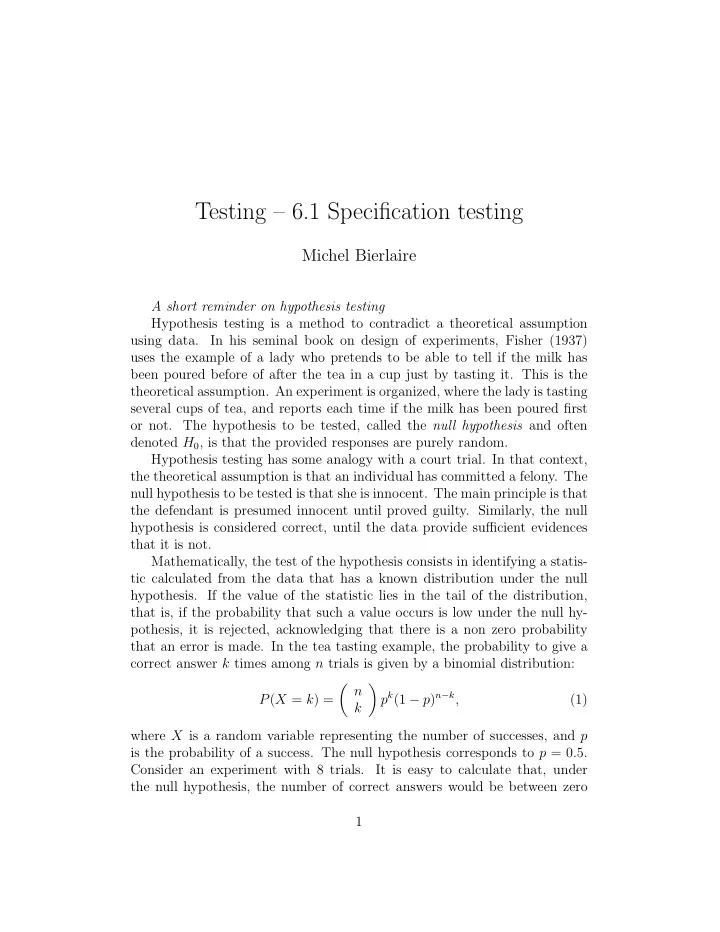
Testing – 6.1 Specification testing Michel Bierlaire A short reminder on hypothesis testing Hypothesis testing is a method to contradict a theoretical assumption using data. In his seminal book on design of experiments, Fisher (1937) uses the example of a lady who pretends to be able to tell if the milk has been poured before of after the tea in a cup just by tasting it. This is the theoretical assumption. An experiment is organized, where the lady is tasting several cups of tea, and reports each time if the milk has been poured first or not. The hypothesis to be tested, called the null hypothesis and often denoted H 0 , is that the provided responses are purely random. Hypothesis testing has some analogy with a court trial. In that context, the theoretical assumption is that an individual has committed a felony. The null hypothesis to be tested is that she is innocent. The main principle is that the defendant is presumed innocent until proved guilty. Similarly, the null hypothesis is considered correct, until the data provide sufficient evidences that it is not. Mathematically, the test of the hypothesis consists in identifying a statis- tic calculated from the data that has a known distribution under the null hypothesis. If the value of the statistic lies in the tail of the distribution, that is, if the probability that such a value occurs is low under the null hy- pothesis, it is rejected, acknowledging that there is a non zero probability that an error is made. In the tea tasting example, the probability to give a correct answer k times among n trials is given by a binomial distribution: � n � p k (1 − p ) n − k , P ( X = k ) = (1) k where X is a random variable representing the number of successes, and p is the probability of a success. The null hypothesis corresponds to p = 0 . 5. Consider an experiment with 8 trials. It is easy to calculate that, under the null hypothesis, the number of correct answers would be between zero 1

and six 96.5% of the time. Therefore, if it happens that seven or eight correct answers are provided, the null hypothesis can be rejected with 3.5% of confidence. If this is not considered sufficient for an evidence, it is possible to be more strict. As there is 99.6% chance to obtain 7 correct answers or less, the analyst could decide to reject the null hypothesis only when 8 correct answers are provided, with confidence 0.4%. The level of confidence is important. Indeed, because of the randomness associated with the data generation process, the outcome of an hypothesis test (that is, rejecting the null hypothesis or not), may be incorrect. There are two types of potential errors, as illustrated in Table 1: • Type I errors occur when the null hypothesis is true, and rejected by the test. Using the analogy with the court trial, it corresponds to sending an innocent to jail. It is sometimes called a “false positive”. We denote α the probability that it occurs: P ( H 0 is rejected | H 0 is true) = α. (2) • Type II errors occur when the null hypothesis is false, but not rejected by the test. Using the analogy with the court trial, it corresponds to releasing a culprit. It is sometimes called a “false negative”. We denote β the probability that it occurs: P ( H 0 is not rejected | H 0 is false) = β. (3) In practice, the analyst decides on α . The value 1 − β , that is P ( H 0 is rejected | H 0 is false) = 1 − β, (4) is called the power of the test. Clearly, for a given data set, decreasing α has the consequence to increase β . The extreme case is to never reject the hypothesis, so that α = 0. Back to our tea tasting example, suppose that the lady has actually the ability to identify if the milk has been poured first or last, with 80% of success rate, and consider again the two tests presented above. 1. The first test rejects the hypothesis when there are 7 or 8 correct an- swers. It fails to reject the (incorrect) null hypothesis β = 49 . 7% of the time (verify using the binomial distribution with p = 0 . 8.) The power of the test is 50.3%. 2

2. The second test rejects the hypothesis when there are 8 correct answers. It fails to reject the (incorrect) null hypothesis β = 83 . 2% of the time. The power of the test is only 16 . 8%. We refer the reader to textbooks in statistics (such as Larsen and Marx (2001, Chapter 6) for a comprehensive introduction to hypothesis testing. Accept H 0 Reject H 0 H 0 is true Type I error (prob. α ) H 0 is false Type II error (prob. β ) Table 1: Type of errors in hypothesis testing References Fisher, R. A. (1937). The design of experiments , Oliver And Boyd, Edinburgh London. Larsen, R. J. and Marx, M. L. (2001). An introduction to mathematical statis- tics and its applications , Vol. 2, 3rd edn, Prentice-Hall, Upper Saddle River, NJ. 3