1. When simulating multiphase flows on fixed grids we must update - - PowerPoint PPT Presentation

DNS of Multiphase Flows Gretar Tryggvason

Direct Numerical Simulations of Multiphase Flows-4
 


Advecting Fluid Interfaces

• 1. When simulating multiphase flows on fixed grids we must update the density and viscosity fields along

with the fluid velocity. This can be done in several different ways and in this segment we will give a brief

• verview of the different strategies most commonly used. In the following lectures we will then describe
• ne approach, front tracking, in more details.

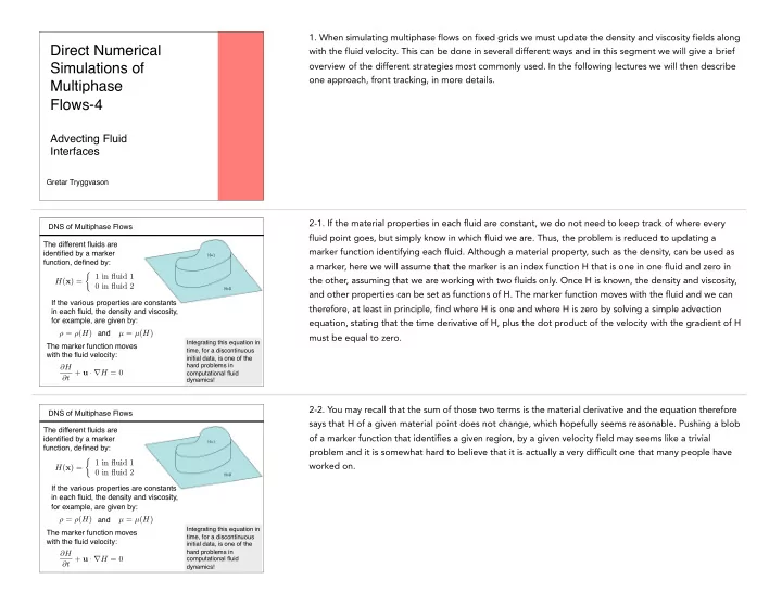
DNS of Multiphase Flows

∂H ∂t + u · rH = 0 ρ = ρ(H) µ = µ(H)

If the various properties are constants in each fluid, the density and viscosity, for example, are given by: The marker function moves with the fluid velocity:

H(x) = ⇢ 1 in fluid 1 0 in fluid 2

and

Integrating this equation in time, for a discontinuous initial data, is one of the hard problems in computational fluid dynamics!

The different fluids are identified by a marker function, defined by:

2-1. If the material properties in each fluid are constant, we do not need to keep track of where every fluid point goes, but simply know in which fluid we are. Thus, the problem is reduced to updating a marker function identifying each fluid. Although a material property, such as the density, can be used as a marker, here we will assume that the marker is an index function H that is one in one fluid and zero in the other, assuming that we are working with two fluids only. Once H is known, the density and viscosity, and other properties can be set as functions of H. The marker function moves with the fluid and we can therefore, at least in principle, find where H is one and where H is zero by solving a simple advection equation, stating that the time derivative of H, plus the dot product of the velocity with the gradient of H must be equal to zero.

DNS of Multiphase Flows

∂H ∂t + u · rH = 0 ρ = ρ(H) µ = µ(H)

If the various properties are constants in each fluid, the density and viscosity, for example, are given by: The marker function moves with the fluid velocity:

H(x) = ⇢ 1 in fluid 1 0 in fluid 2

and

Integrating this equation in time, for a discontinuous initial data, is one of the hard problems in computational fluid dynamics!

The different fluids are identified by a marker function, defined by:

2-2. You may recall that the sum of those two terms is the material derivative and the equation therefore says that H of a given material point does not change, which hopefully seems reasonable. Pushing a blob

• f a marker function that identifies a given region, by a given velocity field may seems like a trivial

problem and it is somewhat hard to believe that it is actually a very difficult one that many people have worked on.

DNS of Multiphase Flows Advecting the marker function using standard methods leads to either excessive smearing for low order methods

• r oscillations when higher order methods are used.

The figure shows the solution of for U =1, computed by a first order upwind method (blue line) and a higher

• rder Lax-Wendroff method

(red line) after propagating 0.6 times the domain length, using 80 grid points to resolve the domain. ∂H ∂t + U ∂H ∂x = 0

0.2 0.4 0.6 0.8 1

• 0.2

0.2 0.4 0.6 0.8 1 1.2 1.4 Exact Lax-Wendroff Upwind

3-1. The obvious question is, of course, why is advecting a blob with a given velocity hard? Can’t we simply take a standard method suitable for the solution of a hyperbolic equation and use that? In the figure we show the results of doing exactly that, for a one-dimensional advection with U equal to 1. We use two standard numerical methods, the first order upwind method and the second order Lax-Wendroff

• method. The initial conditions consist of a step change at the left boundary and the figure shows the

results after the marker function has been advected 0.6 times the domain length to the right, using 80 grid points to resolve the whole domain. The thin black line shows what the solution should look like and it is obvious that neither method does a good job. The blue line shows that the first order method smears out the steep change in H and the higher order method---the red line---produces a solution with large oscillations behind the step. This is what is generally found for linear, or classical, schemes.

DNS of Multiphase Flows Advecting the marker function using standard methods leads to either excessive smearing for low order methods

• r oscillations when higher order methods are used.

The figure shows the solution of for U =1, computed by a first order upwind method (blue line) and a higher

• rder Lax-Wendroff method

(red line) after propagating 0.6 times the domain length, using 80 grid points to resolve the domain. ∂H ∂t + U ∂H ∂x = 0

0.2 0.4 0.6 0.8 1

• 0.2

0.2 0.4 0.6 0.8 1 1.2 1.4 Exact Lax-Wendroff Upwind

3-2. First order methods result in excessive smearing and higher order methods introduce oscillations. While nonlinear schemes have been developed that do a much better job at capturing sharp discontinuities without oscillations, they tend to do very well for shocks in compressible flows and not quite as well for interfaces separating different fluids. Furthermore, since the value on both sides of the discontinuity are known, one is zero and the other one is one, it seems that we should be able come up with methods that do better. This is indeed the case and several methods have been designed for the specific task of advecting a marker function that takes one constant value on one side of the interface and another constant value on the other.

DNS of Multiphase Flows Specialized methods to advect the marker function Volume of Fluid: The average value of the marker function in each cell is updated by computing the flux of markers between cells Level Sets: The interface is identified by the zero contour of a smooth function advected by methods for hyperbolic functions with smooth solutions Front Tracking: The interface is marked by connected marker points that are advected by the fluid velocity interpolated from a fixed grid Both the Level Set and the Front Tracking methods require the construction of the marker function from the interface location

• 4. Of the several methods that have been designed to advect a marker function that takes one constant

value on one side of the interface and another constant value on the other, the best known are the Volume of Fluid method where the average value of the marker function in each cell is updated by computing the flux of markers between cells; the level set method where the interface is identified as the zero contour of a smooth function advected by methods for hyperbolic functions with smooth solutions; and the front tracking method where the interface is marked by connected marker points that are moved by the fluid velocity interpolated from a fixed grid. All of these methods come in several different

• versions. Notice that only in the volume of fluid method is the marker function updated directly and that

in both the level set and the front tracking method we need to construct the marker function from the interface location.

DNS of Multiphase Flows The sharp marker function H can be approximated in several different ways for computational purposes. Below we show a smoothed marker function, I, the volume of fluid approximation, C, and a level set representation, Φ. Advecting the Marker Function Interface cell

j-1 j j+1 j-1/2 j+1/2

ϕ(x) I(x) H(x) Cj

• 5. Although the methods listed on the previous slide have much in common, they differ in exactly what is

advected and how the marker function is approximated. In the Volume of Fluid method we work with the average value of the marker in each computational cell and advect the marker directly. In the figure this is shown by C, which has a constant value everywhere, either 0 or 1, except in the interface cell j. In level set methods we advect a smooth functions, phi of x---shown by a nearly straight dashed dot line in the figure---which crosses the zero axis where the interface is located. And in front tracking methods we advect a point that is located exactly where the interface is, or where the discontinuity in H is. We do, however, need a marker function so for both level set and front tracking methods this needs to be constructed from the interface location. Although the construction of the marker function is different, in both methods the marker is generally taken to have a smooth transition from one constant value to the next, so that it looks like the dashed line, shown by I of x, in the figure. We now take a slightly closer look at these methods.

DNS of Multiphase Flows

Volume of Fluid

• 6. The Volume of Fluid method is the most widely used approach to update the marker function. In one

dimension the advection of a sharp discontinuity separating regions of constant value is exact. This makes it a natural starting point for multidimensional problems, but unfortunately the extension to higher dimensions is far from trivial and requires making rather significant approximations.

DNS of Multiphase Flows Upwind To advect a discontinuous marker function, first consider 1D

• advection. Using simple upwind leads to excessive diffusion

due to averaging the function over each cell, before finding the fluxes. The remedy is to compute the fluxes more accurately such that nothing flows into cell j+1 until cell j is full

j-1 j j+1 Cj-1 Cj Cj+1 U j-1 j j+1 UΔt j-1 j j+1 Cj-1 Cj Cj+1

• 7. The challenge of advecting a marker function using a standard finite volume method is best

introduced by an example. Consider the situation in the first figure. The interface is located in the middle cell and since we only keep the average value of the marker function the cell is half full. By itself, the average value does not specify the exact location of the interface since in general there are two possibilities, depending of whether fluid 1 is located to the left or right of the interface. To update the marker we compute the flux of the marker through the cell boundary and for the linear advection equation this is easily done. Indeed, given the initial conditions we simply move the marker with a constant velocity to the left or right, depending on the sign of the velocity. If the velocity is positive, the marker moves to the right and we update the marker by moving everything a distance U delta t to the right, as shown in the middle frame, and then average as shown in the frame on the right. Unfortunately, the interface is now spread over two cells and if we continue the process the interface will continue to spread out, or diffuse, over more and more cells.

DNS of Multiphase Flows One-dimensional Volume-Of-Fluid Since the marker function only takes on two values, 0 and 1, the advection can be made much more accurate by “reconstructing” the function in each cell before finding the fluxes, integrated over time:

Z ⇢

• Z t+∆t

t

Fj+1/2 dt = ⇢ 0, if ∆t  (1 Cj)∆x/U, ∆x (Cj + U∆t), if ∆t > (1 Cj)∆x/U

j-1 j j+1 Cj-1 Cj Cj+1 U j-1 j j+1 UΔt j-1 j j+1 Cj-1 Cj Cj+1

8-1. The problem, obviously, is that we took the initial conditions to be the average value in the cell so when we move the marker to the right, the cell on the right of the interface cell starts to receive marker, even if the middle cell is not full. The solution is to look to the neighboring cells, determine that the marker is non-zero on the left (in this case) and use that to reconstruct more realistic initial conditions. It is, in particular, easy to determine exactly where the interface is. If the value is C_j, then the interface is C_j times delta x from the left boundary and if the size of the time step is such that the interface moves less than 1-C_j times delta x, or when U delta t is less than 1-C_j delta x, then nothing should flow into the cell on the right. If the time is greater, or if U delta t is greater than 1-C_j times delta x then the total amount of C that flows from cell j to cell j+1 is U delta t minus the amount of C that remained in cell j, or delta x minus C_j times U delta t.

DNS of Multiphase Flows One-dimensional Volume-Of-Fluid Since the marker function only takes on two values, 0 and 1, the advection can be made much more accurate by “reconstructing” the function in each cell before finding the fluxes, integrated over time:

Z ⇢

• Z t+∆t

t

Fj+1/2 dt = ⇢ 0, if ∆t  (1 Cj)∆x/U, ∆x (Cj + U∆t), if ∆t > (1 Cj)∆x/U

j-1 j j+1 Cj-1 Cj Cj+1 U j-1 j j+1 UΔt j-1 j j+1 Cj-1 Cj Cj+1

8-2. The flux through the right boundary of the middle cell is therefore zero if delta t is less than 1-C_j times delta x, divided by U, and delta x minus C_j plus U times delta t if delta t is greater than 1-C_j times delta x, divided by U. The flux into the cell is simply U times delta t, since C in the j-1 cell is equal to 1. The key here is that we located the interface exactly by examining the neighboring cells and this allowed us to write down the exact flux in such a way that the cells fill up one by one and no diffusion takes place.

DNS of Multiphase Flows While VOF works extremely well in one-dimension, there are considerable difficulties extending the approach to higher dimensions. The basic problem is the “reconstruction” of the interface in each cell, given the volume fraction in neighboring cells. In the Simple Line Interface Calculations or SLIC method the interface was taken to be perpendicular to the advection direction. In the Hirt/Nichols method the interface was taken to be parallel to one axis. In Piecewise Linear Interface Calculations or PLIC the interface is a line with arbitrary orientation.

9-1. The simplest extension of this straightforward method to two and three-dimensions is to do the advection in one direction at a time, using the one-dimensional formulation. In this approach, known as the Simple Line Interface Calculation or SLIC, we construct a horizontal interface for advection in the vertical direction, followed by constructing a vertical interface for advection in the horizontal direction. The problem with this approach is that the cells on either side of the interface cell are not always full or completely empty and not only does that introduce uncertainty in locating the interface but the interface can also break up due to the generation of partially full cells away from the interface. In an effort to improve the SLIC method, Hirt and Nichols suggested that the interface in each cell should be approximated as either a vertical or horizontal one, based on a normal vector estimated by considering the volume fraction in neighboring cells. While this did not result in a significant improvement, it suggested that an interface reconstruction based on the normal might lead to better results.

DNS of Multiphase Flows While VOF works extremely well in one-dimension, there are considerable difficulties extending the approach to higher dimensions. The basic problem is the “reconstruction” of the interface in each cell, given the volume fraction in neighboring cells. In the Simple Line Interface Calculations or SLIC method the interface was taken to be perpendicular to the advection direction. In the Hirt/Nichols method the interface was taken to be parallel to one axis. In Piecewise Linear Interface Calculations or PLIC the interface is a line with arbitrary orientation.

9-2. This is, indeed, the case and the next improvement was the Piecewise Linear Interface Calculation method or PLIC, where the interface is assumed to consist of a line whose orientation is based on an estimation of the normal to the interface and whose location is adjusted such that the average value of the marker in the interface cell is correct. This improved considerably the performance of Volume of Fluid methods, but at the cost of much more complex flux calculations.

DNS of Multiphase Flows Original SLIC PLIC Hirt/Nichols VOF

• 10. This slide shows the various version of the Volume of Fluid method schematically. The configuration
• f the fluid interface and the grid used to represent the field is shown in the upper left corner. The
• riginal split VOF method, the SLIC method is shown in the upper right corner, where the solid and the

dashed line show the orientation for advection in the different directions. The Hirt and Nichols method, where the interface in each cell is assumed to be either vertical or horizontal is shown in the lower left corner and finally, the PLIC method, where the interface is approximated by a sloping line that may be discontinuous at cell boundaries, is shown in the lower right corner. More sophisticated VOF methods are continuously being developed and many of those do an excellent job of following sharp interfaces.

DNS of Multiphase Flows There are many versions of PLIC, but in all cases the steps are: 1.Given the value of the marker function in each cell, estimate the normal.

• 2. Given the value of the marker function in each cell

and the normal, reconstruct the interface (slope and location of the line bisecting the control volumes with fractional values of the marker function).

• 3. Advect the marker function and find the value of the

marker function in each cell at the next time step.

• 11. There are many versions of PLIC, but in all cases the first step is to estimate the normal vector in each

cell, given the value of the marker function in the cell that we are considering and in the neighboring

• cells. Once we have the normal, we draw a line perpendicular to the normal and move it in the direction
• f the normal until the area cut out from the interface cell by the line matches the value of the marker

function in the cell. Knowing the shape of the region occupied by the marker function in each interface cell then allows us to advect the marker using geometric considerations.

DNS of Multiphase Flows Given the volume fraction in each cell, we start by finding the normals. This can be done in several ways, but here we use simple centered differences of the volume fractions. In many cases smoother approximations are used or the results are averaged over a few cells.

C(i,j)=0.933 C(i-1,j)=1.000 C(i+1,j)=0.249 C(i-1,j+1) = 0.715 C(i,j+1) = 0.091 C(i+1,j+1) = 0.000 nx(i, j) = C(i + 1, j) C(i 1, j) 2∆x ny(i, j) = C(i, j + 1) C(i, j 1) 2∆y

• 12. The normal can be found in many ways but in most cases it is estimated to be the gradient of the

marker function. Since the marker function changes abruptly from one to zero over only one cell, some smoothing is generally involved, but the simplest approximation is to use centered differences as shown

• here. Notice that both the interface cells and cells close to the interface have a non-zero normal.

DNS of Multiphase Flows Interface is moved along the normal to give the correct value of the marker in the cell under consideration Once the normal has been determined, the location of the interface is adjusted to give the correct value of the volume fraction of the marker in the cell. The normal and the fractional value of the marker in the interface cell determine the shape of the region occupied by the marker in each cell The normal to the interface

• 13. Once the normal is found, the slope of the interface is known. We approximate the interface by a

straight line perpendicular to the normal and the location of the interface is found by moving it along the normal until the area below the interface matches the volume fraction of marker, in the interface cell.

DNS of Multiphase Flows The marker function can be advected in many ways. The simplest is to move the marker first in one direction and then in the other, assuming that the velocity remains constant during the time step. Here we consider a velocity advecting the marker in the positive x and y directions.

U

u v

Full cell Full cell

i-1,j-1 i,j i-1,j i,j-1 i,j+1 i+1,j

• 14. The marker can be advected in several ways but the simplest approach is to advect it first in one

direction and then in the other. Consider the cell shown in the figure, where the interface cuts through the top and the right side of the cell and the cells to the left and below are full. If we assume that the velocity remains constant during the time step then advection in the x-direction corresponds to shifting everything in the cell a distance equal to u times delta t, where u is the x-component of the velocity.

DNS of Multiphase Flows Here, the gray region at the right will move out of cell i,j and the gray region at the left will move into cell i,j.

U

u v uΔt uΔt

i-1,j-1 i,j i-1,j i,j-1 i,j+1 i+1,j

The marker function can be advected in many ways. The simplest is to move the marker first in one direction and then in the other, assuming that the velocity remains constant during the time step. Here we consider a velocity advecting the marker in the positive x and y directions.

• 15. Here, the gray region on the right will move out of cell i,j and the gray region on the left will move

into cell i,j.

DNS of Multiphase Flows Marker advected from cell i-1,j into cell i,j during advection in the x-direction

U

u v

Marker advected from cell i,j into cell i+1,j during advection in the x-direction Marker advected from cell i-1,j-1 into cell i,j-1 during advection in the x-direction

i-1,j-1 i,j i-1,j i,j-1 i,j+1 i+1,j

• 16. Thus, the total amount of marker that flows into cell i,j from the cell on the left, i-1,j, is given by the

gray tall rectangle on the left and the total amount of marker that flows out of cell i,j into cell i+1,j on the right is given by the gray polygon on the right.

DNS of Multiphase Flows The advection in the y- direction is done in the same way. The interfaced is reconstructed again and the regions that will move into new cells identified. Here, the gray region at the top will move out of cell i,j and the gray region at the bottom will move into cell i,j.

U

u v vΔt

i-1,j-1 i,j i-1,j i,j-1 i,j+1 i+1,j

vΔt

• 17. The advection in the y-direction is done in the same way. The interfaced is reconstructed from the

fraction of the marker in the interface cell and the normal vector, computed using the amount of marker in the neighboring cells, and the regions that will move into new cells are identified. Here, the gray region at the top will move out of cell i,j and the gray region at the bottom will move into cell i,j.

DNS of Multiphase Flows Marker advected from cell i,j into cell i,j+1 during advection in the y-direction Marker advected from cell i-1,j-1 into cell i,j by advecting first in the x direction and then in the y direction Marker advected from cell i,j-1 into cell i,j during advection in the y-direction

i-1,j-1 i,j i-1,j i,j-1 i,j+1 i+1,j

• 18. The total amount of marker that flows into cell i,j from the cell on the bottom, i,j-1, is given by the

gray wide rectangle at the bottom and the total amount of marker that flows out of cell i,j into cell i,j+1 is given by the gray polygon on the top.

DNS of Multiphase Flows To maintain symmetry with respect to x and y, the order

• f advection is usually alternated.

This simple scheme conserves the marker function C, but does not guarantee that it remains bounded between 0 and 1. More advanced method conserve C and ensure that 0<C<1. For fully three-dimensional schemes both the reconstructing of the interface as well as the advection requires careful considerations of the interface geometry

• 19. To maintain symmetry with respect to x and y, the order of advection is usually alternate. [Pause] The

approach described here conserves the marker function C, since what flows out of one cell flows into another cell, but does not guarantee that it remains bounded between 0 and 1. However, more advanced methods exists that both conserve C and ensure that it is bounded between 0 and 1. For fully three-dimensional schemes both the reconstruction of the interface, as well as the advection, are considerably more complex and require careful considerations of the interface geometry

DNS of Multiphase Flows

Level Set Methods

• 20. Given how difficult it is to advect a sharp interface in multi-dimensions, we might ask why bother with

a sharp interface, at all? The interface can be identified as a constant value contour of a smooth function and it is much easier to advect smooth fields than discontinuous ones. This is the idea behind the Level Set method.

DNS of Multiphase Flows Identify the interface as a “level- set” of a smooth function Advect the level set function by use to get

∂φ ∂t + u · rφ = 0 |r | ∂φ ∂t + un|rφ| = 0 n = rφ |rφ| u · n = un

• 21. In the level set method we identify the interface with a given value (usually taken to be zero) of a

smooth function phi. Phi is then advected with the fluid and since the interface is a material point, the zero contour, or the level set, is advected as well. Since it is only the normal velocity that matters, the advection equation is usually rewritten by using that the unit normal to the interface can be found as the gradient of the level set function divided by the magnitude of the gradient, and that the velocity dotted into the unit normal is the normal velocity. Wherever the level set function phi is zero, there is an interface, and for the two-peaked function shown here, there are two closed interfaces since two peaks stick out through the zero plane.

DNS of Multiphase Flows The level set function can be arbitrarily smooth. To identify each fluid it is necessary to construct a marker function with a narrow transition zone The marker function can be generated by (for example): The delta function is generated as the derivative

• f the marker function

δ = rI = dI dφrφ

I(φ) = 8 < : if φ < α∆x

1 2(1 + φ α∆x + 1 π sin(π φ α∆x)

if |φ|  α∆x 1 if φ > α∆x

I(φ) φ

we need is to update the marker function. The zero level set only gives us the location of the interface. Thus, we need to map the smooth level set function into a marker function that changes rapidly, but smoothly, from one constant value to another constant value. Furthermore, we generally want the shape

• f the transition zone to remain more or less the same everywhere and at all times. If the shape of the

level set function in the vicinity of the zero contour remained the same this would be easily accomplished and we could simply pick a mapping function, such as the sine function shown here. Once the marker function has been determined, we can obviously also find a smooth approximation to the delta function by differentiation. This can obviously be related to the level set function as shown at the bottom of the slide.

DNS of Multiphase Flows The distortion makes the transition zone from one level of the marker function to the other depend on the history of the flow For most applications, the shape of the level set functions must remain the same close to the interface so that the width

• f the transition zone for the indicator function remains

approximately constant. The flow does, however, usually distort the shape

• 23. Unfortunately the level set function is generally distorted significantly by non-uniform flows around

the interface. If the interface is being stretched, for example, the gradient of the level set function increases and if it is compressed the gradient decreases, making the level set function flatter. In the example here, where we have stagnation point flow on the left, the level set function is compressed, making the transition in the marker function steeper and on the right, where the flow is reversed, the transition zone becomes thicker.

DNS of Multiphase Flows Usually only a few “time steps” are necessary since the level set function only has to be corrected near the interface. To keep the interface shape the same, the level set function is “reinitialized” once in a while. This is usually done by making it a distance function, where . This can be enforced by solving in ‘pseudo” time . ∂φ ∂τ + sgn(φ)(|rφ| 1) = 0

|rφ| = 1

τ

• 24. In order to make the marker function transition from one value to the other in the same way

everywhere, the level set function must be reset in such a way that its slope is always the same next to the interface. In the original level set method this was achieved by reinitializing the level set function so that it remained a distance function, whose value was equal to the shortest distance to the interface. The gradient of a distance function is normal to the interface and should remain unity, for the level set function to remain a distance function. This can be done by setting the difference between the absolute value of the gradient and unity equal to the time derivative of level set function and solving it in pseudo time where the interface remains stationary and the real time is frozen. Obviously, if the time derivative is zero, then the absolute value of the gradient is equal to unity. The sign function accounts for the fact that the level set function changes sign across the interface but the gradient does not. Usually we are only concerned with the shape of the level set function close to the interface and we only need to solve the re-initialization equation to correct the shape there.

DNS of Multiphase Flows

Front-Tracking Methods

• 25. Unlike the VOF method where the marker function is updated directly, in the level set method the

update of the marker function is a two-step process. First, the interface is advected and second, the marker function is constructed from the smooth function. Front tracking is also a two-step process where the interface is first moved and the marker function is then constructed. The identification of the interface and how it is moved is, however, very different.

DNS of Multiphase Flows

The interface is identified by connected marker particles that are advcted by the fluid velocity, interpolated from the grid used to solve the Navier-Stokes equations The marker particles and their connections are usually referred to as the FRONT The marker function is then constructed from the location of the front and used to set the density and the viscosity The front is also used to compute surface tension, which must be distributed to the fixed grid and added to the Navier Stokes equations The front usually deforms as the flow evolves and must be modified by adding and deleting points and elements

• 26. In its simplest embodiment the interface in Front Tracking is represented by connected marker

particles that move with the fluid velocity. For two-dimensional flows the front is simply a string of points, but in three-dimensions the front is a two-dimensional surface that needs to be represented by a surface grid of some sort to account for the connectivity of the markers. The marker particles and the connections are usually referred to as the front. The marker particles are advcted by the fluid velocity, interpolated from the grid used to solve the Navier-Stokes equations. The marker function is then constructed from the location of the front and used to set the density and the viscosity. The front is also used to compute surface tension, which must be distributed to the fixed grid and added to the Navier Stokes equations. The front usually deforms as the flow evolves and must be modified by adding and deleting marker points.

DNS of Multiphase Flows

Fixed grid used for the solution of the Navier-Stokes equations. Relatively standard explicit finite volume fluid solver Tracked front consisting of marker points connected by triangular elements, forming an unstructured grid, used to advect the marker function and find surface tension The front management, adding and deleting points, as well as changing the topology of the front when needed, are generally considered the main challenges with front tracking

• 27. Here we show the front and the fixed grid used to solve the Navier-Stokes equations. The fluid solver

is usually a relatively standard finite volume method implemented on a regular structured grid, although as with the level set and the volume of fluid method we can in principle use any flow solver. For three- dimensional flow the interface is an imbedded two-dimensional surface, and since its geometry can be fairly complex, we usually use an unstructured grid, typically consisting of points that are connected by triangular elements. Generally the size of the triangular elements is some fraction of the size of the control volumes used for the fluid flow and as the flow evolves, the unstructured two-dimensional grid is deformed, stretched and compressed. Thus, it is usually necessary to update the grid once in a while to maintain the resolution. This updating, where we need to add and delete points and elements and sometimes change the topology is generally considered the main challenges with front tracking. In the next lecture we will focus on two-dimensional flow where the front is simply a one-dimensional curve and adding and deleting points is relatively simple.

DNS of Multiphase Flows

Implementation of front tracking methods require several

• steps. The major ones are:

The front is moved by the fluid velocities, interpolated from the fixed grid The marker function is constructed from the front The front is used to compute surface tension which is then smoothed onto the fixed grid All these operations can be done in a number of different

• ways. We will introduce one relatively simple approach in the

next few lectures. The implementation focuses on two- dimensional flows, which are considerably simpler than fully three-dimensional ones. However, the underlying ideas remain the same

• 28. Implementation of front tracking methods requires several steps. We usually move the front with the

fluid velocities, which must be interpolated from the fixed grid used to solve the Navier-Stokes equations; then we need to construct a marker function from the location of the front; and for immiscible fluids we need to find the surface tension from the front geometry and add it to the discrete Navier- Stokes equations on the fixed grid. We can do these operations in several different ways and in the next lectures we will work through one relatively simple approach. Although our implementation focuses on two-dimensional flows, which are considerably simpler than fully three-dimensional ones, the underlying ideas remain the same.

DNS of Multiphase Flows

Several other methods have been developed to improve the performance of those described here, including hybrid methods, such as Particle Level Set and VOF-LS, as well as methods that capture the interface more sharply, such as the Ghost Fluid Method and the Immersed Interface Method. Similar approach has also been used to capture rigid and elastic boundaries, both moving and stationary.

• 29. Hybrid methods, such as Particle Level Set and combined Volume of Fluid Level Set methods, as well

as methods that capture the interface more sharply, such as the Ghost Fluid Method and the Immersed Interface Method. Considerable effort has also been devoted to the development of similar approaches to capture rigid and elastic boundaries, both moving and stationary. Of the elementary methods described in this lecture, front tracking appears to be the most robust and accurate approach and while work on both level set and volume of fluid methods continues, the front tracking approach described here is still often used in more or less its original form. In the next lectures we will describe a simple implementation in sufficient detail so that we can code it up.