Volume of Fluid j- 1/2 j+ 1/2 H ( x ) C j I ( x ) ( x ) j -1 j j +1 - PDF document


 DNS of Multiphase Flows DNS of Multiphase Flows Direct Numerical The different fluids are Simulations of identified by a marker function, defined by: Multiphase ⇢ 1 in fluid 1 H ( x ) = 0 in fluid 2 Flows-4 
 If the various properties are constants in each fluid, the density and viscosity, for example, are given by: Advecting Fluid ρ = ρ ( H ) and µ = µ ( H ) Interfaces Integrating this equation in The marker function moves time, for a discontinuous with the fluid velocity: initial data, is one of the hard problems in ∂ H Gretar Tryggvason ∂ t + u · r H = 0 computational fluid dynamics! DNS of Multiphase Flows DNS of Multiphase Flows Specialized methods to advect the marker function Advecting the marker function using standard methods leads to either excessive smearing for low order methods Volume of Fluid: The average value of the marker function in or oscillations when higher order methods are used. 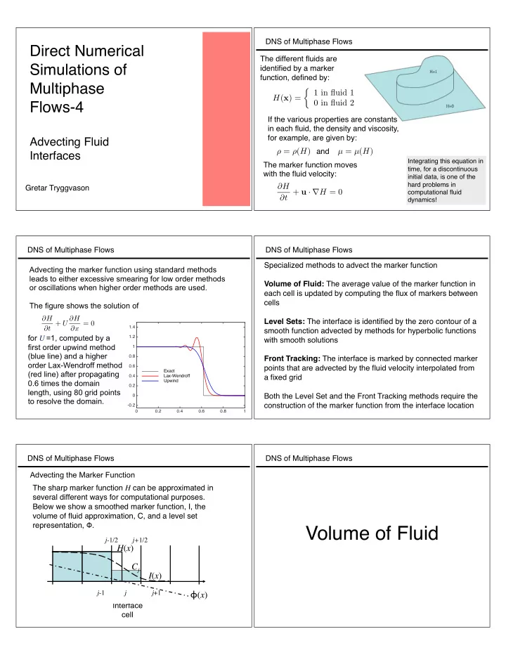each cell is updated by computing the flux of markers between cells The figure shows the solution of ∂ H ∂ t + U ∂ H Level Sets: The interface is identified by the zero contour of a ∂ x = 0 1.4 smooth function advected by methods for hyperbolic functions for U =1, computed by a 1.2 with smooth solutions first order upwind method 1 (blue line) and a higher 0.8 Front Tracking: The interface is marked by connected marker order Lax-Wendroff method 0.6 points that are advected by the fluid velocity interpolated from Exact (red line) after propagating 0.4 Lax-Wendroff a fixed grid 0.6 times the domain Upwind 0.2 length, using 80 grid points Both the Level Set and the Front Tracking methods require the 0 to resolve the domain. construction of the marker function from the interface location -0.2 0 0.2 0.4 0.6 0.8 1 DNS of Multiphase Flows DNS of Multiphase Flows Advecting the Marker Function The sharp marker function H can be approximated in several different ways for computational purposes. Below we show a smoothed marker function, I, the volume of fluid approximation, C, and a level set representation, Φ . Volume of Fluid j- 1/2 j+ 1/2 H ( x ) C j I ( x ) ϕ ( x ) j -1 j j +1 Interface cell

DNS of Multiphase Flows DNS of Multiphase Flows To advect a discontinuous marker function, first consider 1D Since the marker function only takes on two values, 0 and 1, advection. Using simple upwind leads to excessive diffusion the advection can be made much more accurate by due to averaging the function over each cell, before finding “reconstructing” the function in each cell before finding the the fluxes. fluxes, integrated over time: ⇢ Z � � The remedy is to compute the fluxes more accurately such Z t + ∆ t ⇢ 0 , if ∆ t  (1 � C j ) ∆ x/U, F j +1 / 2 dt = that nothing flows into cell j +1 until cell j is full ∆ x � ( C j + U ∆ t ) , if ∆ t > (1 � C j ) ∆ x/U t One-dimensional Volume-Of-Fluid Upwind U U Δ t U U Δ t C j -1 C j C j +1 C j -1 C j C j +1 C j -1 C j C j +1 C j -1 C j C j +1 j -1 j j +1 j -1 j j +1 j -1 j j +1 j -1 j j +1 j -1 j j +1 j -1 j j +1 DNS of Multiphase Flows DNS of Multiphase Flows While VOF works extremely well in one-dimension, there are considerable difficulties extending the approach to higher dimensions. The basic problem is the Original SLIC “reconstruction” of the interface in each cell, given the volume fraction in neighboring cells. In the Simple Line Interface Calculations or SLIC method the interface was taken to be perpendicular to the advection direction. In the Hirt/Nichols method the interface was taken to be parallel to one axis. Hirt/Nichols PLIC In Piecewise Linear Interface Calculations or PLIC the VOF interface is a line with arbitrary orientation. DNS of Multiphase Flows DNS of Multiphase Flows Given the volume There are many versions of PLIC, but in all cases the fraction in each cell, we steps are: start by finding the C ( i+1,j+1 ) C ( i-1,j+1 ) C ( i,j+1 ) normals. = 0.000 = 0.715 = 0.091 1.Given the value of the marker function in each cell, estimate the normal. This can be done in several ways, but here 2. Given the value of the marker function in each cell we use simple centered and the normal, reconstruct the interface (slope and differences of the C ( i-1,j )=1.000 C ( i,j )=0.933 C ( i+1,j )=0.249 location of the line bisecting the control volumes with volume fractions. fractional values of the marker function). In many cases smoother approximations are n x ( i, j ) = C ( i + 1 , j ) � C ( i � 1 , j ) 3. Advect the marker function and find the value of the used or the results are 2 ∆ x marker function in each cell at the next time step. averaged over a few n y ( i, j ) = C ( i, j + 1) � C ( i, j � 1) cells. 2 ∆ y

DNS of Multiphase Flows DNS of Multiphase Flows The normal to the interface Once the normal has been The marker function can be i,j+ 1 determined, the location of the advected in many ways. interface is adjusted to give The simplest is to move the the correct value of the marker first in one direction volume fraction of the marker Full and then in the other, i,j in the cell. cell i+ 1 ,j assuming that the velocity v U The normal and the fractional remains constant during i- 1 ,j value of the marker in the the time step. u interface cell determine the Here we consider a velocity Full cell shape of the region occupied advecting the marker in the i- 1 ,j- 1 i,j- 1 by the marker in each cell positive x and y directions. Interface is moved along the normal to give the correct value of the marker in the cell under consideration DNS of Multiphase Flows DNS of Multiphase Flows u Δ t u Δ t The marker function can be i,j+ 1 i,j+ 1 advected in many ways. Marker advected from cell i-1,j into cell i,j during The simplest is to move the advection in the x-direction marker first in one direction and then in the other, i,j i,j i+ 1 ,j i+ 1 ,j assuming that the velocity v v U U remains constant during Marker advected from cell i- 1 ,j i- 1 ,j i,j into cell i+1,j during the time step. u u advection in the x-direction Here we consider a velocity advecting the marker in the i- 1 ,j- 1 i- 1 ,j- 1 i,j- 1 i,j- 1 positive x and y directions. Marker advected from cell i-1,j-1 into cell Here, the gray region at the right will move out of cell i,j and i,j-1 during advection in the x-direction the gray region at the left will move into cell i,j. DNS of Multiphase Flows DNS of Multiphase Flows The advection in the y- i,j+ 1 i,j+ 1 Marker advected from cell i,j direction is done in the into cell i,j+1 during advection same way. in the y-direction v Δ t The interfaced is reconstructed again and i,j i,j i+ 1 ,j i+ 1 ,j the regions that will move v U into new cells identified. i- 1 ,j i- 1 ,j Marker advected from cell u Here, the gray region at i,j-1 into cell i,j during the top will move out of v Δ t advection in the y-direction cell i,j and the gray region i- 1 ,j- 1 i- 1 ,j- 1 i,j- 1 i,j- 1 at the bottom will move into cell i,j. Marker advected from cell i-1,j-1 into cell i,j by advecting first in the x direction and then in the y direction

DNS of Multiphase Flows DNS of Multiphase Flows To maintain symmetry with respect to x and y , the order of advection is usually alternated. This simple scheme conserves the marker function C , but does not guarantee that it remains bounded between Level Set 0 and 1 . More advanced method conserve C and ensure that Methods 0< C <1 . For fully three-dimensional schemes both the reconstructing of the interface as well as the advection requires careful considerations of the interface geometry DNS of Multiphase Flows DNS of Multiphase Flows Identify the interface as a “level- The level set function can be arbitrarily smooth. To identify set” of a smooth function each fluid it is necessary to construct a marker function with a narrow transition zone Advect the level set function by The marker function can be generated by (for example): ∂φ 8 0 if φ < � α ∆ x ∂ t + u · r φ = 0 < φ φ I ( φ ) = 1 α ∆ x + 1 2 (1 + π sin( π α ∆ x ) if | φ |  α ∆ x 1 if φ > α ∆ x : use The delta function is n = r φ I ( φ ) u · n = u n generated as the derivative | r φ | of the marker function to get | r | δ = r I = dI d φ r φ ∂φ ∂ t + u n | r φ | = 0 φ DNS of Multiphase Flows DNS of Multiphase Flows For most applications, the shape of the level set functions To keep the interface shape the same, the level set function must remain the same close to the interface so that the width is “reinitialized” once in a while. This is usually done by of the transition zone for the indicator function remains making it a distance function, where . This can be | r φ | = 1 approximately constant. The flow does, however, usually enforced by solving distort the shape ∂φ ∂τ + sgn( φ )( | r φ | � 1) = 0 in ‘pseudo” time . τ The distortion makes the transition zone from one level of the Usually only a few “time steps” are necessary since the level marker function to the other depend on the history of the flow set function only has to be corrected near the interface.