1. One of the major challenges in simulating multiphase flows is - - PowerPoint PPT Presentation

▶

Nov 02, 2023 550 likes •625 views

1. One of the major challenges in simulating multiphase flows is the advection of the marker function DNS of Multiphase Flows Simple Front Tracking Direct Numerical that identifies the different fluids. There are two main ways to do so:

SLIDE 1

DNS of Multiphase Flows — Simple Front Tracking

Direct Numerical Simulations of Multiphase Flows-5   

Advecting the Marker Function using Front Tracking (1 of 2)

Gretar Tryggvason

1. One of the major challenges in simulating multiphase flows is the advection of the marker function

that identifies the different fluids. There are two main ways to do so: We can update the marker function directly by solving an advection equation, or we can move the interface separating the different fluids and then reconstruct the marker function from the location of the interface. Here we do the latter by placing connected marker points at the interface, and then moving them with the flow.

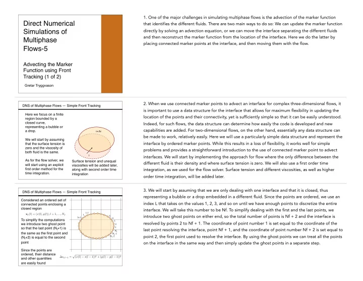
DNS of Multiphase Flows — Simple Front Tracking Here we focus on a finite region bounded by a closed curve, representing a bubble or a drop. We will start by assuming that the surface tension is zero and the viscosity of both fluid is the same. As for the flow solver, we will start using an explicit first order method for the time integration.

t+Δt" t"

Surface tension and unequal viscosities will be added later, along with second order time integration

2. When we use connected marker points to advect an interface for complex three-dimensional flows, it

is important to use a data structure for the interface that allows for maximum flexibility in updating the location of the points and their connectivity, yet is sufficiently simple so that it can be easily understood. Indeed, for such flows, the data structure can determine how easily the code is developed and new capabilities are added. For two-dimensional flows, on the other hand, essentially any data structure can be made to work, relatively easily. Here we will use a particularly simple data structure and represent the interface by ordered marker points. While this results in a loss of flexibility, it works well for simple problems and provides a straightforward introduction to the use of connected marker point to advect

interfaces. We will start by implementing the approach for flow where the only difference between the

different fluid is their density and where surface tension is zero. We will also use a first order time integration, as we used for the flow solver. Surface tension and different viscosities, as well as higher

rder time integration, will be added later.

DNS of Multiphase Flows — Simple Front Tracking Considered an ordered set of connected points enclosing a closed region To simplify the computations we introduce two ghost point so that the last point (Nf+1) is the same as the first point and (Nf+2) is equal to the second point Since the points are

rdered, their distance

and other quantities are easily found

1! 2! 3! Nf! Nf -1! Nf -2! 4! 5! l! l-1! l+1!

xf(l) = (x(l), y(l)), l = 1, ...., Nf ∆sl,l−1 = p (x(l) − x(l − 1))2 + (y(l) − y(l − 1))2

3. We will start by assuming that we are only dealing with one interface and that it is closed, thus

representing a bubble or a drop embedded in a different fluid. Since the points are ordered, we use an index L that takes on the values 1, 2, 3, and so on until we have enough points to discretize the entire

interface. We will take this number to be Nf. To simplify dealing with the first and the last points, we

introduce two ghost points on either end, so the total number of points is Nf + 2 and the interface is resolved by points 2 to Nf + 1. The coordinate of point number 1 is set equal to the coordinate of the last point resolving the interface, point Nf + 1, and the coordinate of point number Nf + 2 is set equal to point 2, the first point used to resolve the interface. By using the ghost points we can treat all the points

n the interface in the same way and then simply update the ghost points in a separate step.

SLIDE 2

DNS of Multiphase Flows — Simple Front Tracking

%================== SETUP THE FRONT =================== Nf=100; xf=zeros(1,Nf+2);yf=zeros(1,Nf+2); uf=zeros(1,Nf+2);vf=zeros(1,Nf+2); tx=zeros(1,Nf+2);ty=zeros(1,Nf+2); for l=1:Nf+2, xf(l)=xc-rad*sin(2.0*pi*(l-1)/(Nf)); yf(l)=yc+rad*cos(2.0*pi*(l-1)/(Nf)); end 1 2 (xc,yc)

Here we construct a circle, starting at the top and going counter clockwise. Notice that there are ghost points at both ends so that we run over the points by: for l=2:Nf+1 …. end and then set the values at 1 and Nf+2

Nf Nf+1 Nf+2 Nf-1 3 rad θ

4. If the initial shape of the interface is a circle, its construction is particularly easy. Once we have decided

where the center of the circle, xc and yc, is, where we start and in what direction to go, the coordinates are easily found. We can obviously start anywhere and go either clockwise or counter clockwise, but here we start directly above the center and go in the counter clockwise direction. The x coordinate is given as the x coordinate of the center minus the radius times the sine of the angle from the vertical axis, and the y coordinate is then given by the y coordinate of the center plus the radius times the cosine of the angle from the vertical axis. The angle increment is two pi divided by the number of points used to resolve the interface, Nf-1, and we increment it by l-1, where l is the point number, since we want to start with a zero angle so that the first point is directly above the center.

DNS of Multiphase Flows — Simple Front Tracking

Transferring information between the front and the grid

5. Since we are using two grids, the fixed regular structured two-dimensional grid where we solve the

fluid equations and the one-dimensional moving grid, which we use to mark the interface and construct the density and the surface tension, we need to transfer information between those two grids.

DNS of Multiphase Flows — Simple Front Tracking To transfer information between the front and the fixed grid, we need to find the grid point closest to the front The index of the point to the left

f the front location is given by

0 1 2 3 4 5 nx

Horizontal Velocity (u) Left Boundary Front Location Right Boundary p i = FLOOR(xf(l)/∆x) + 1

Control volume boundary Grid points where the velocity is stored

The velocity at the front is interpolated to the points on the left and the right

6. The easiest way is to start with a point on the interface and ask what point on the fixed grid is closest.

This, as we will emphasize again later, is a much simpler problem than asking what interface point is closest to a given grid point! Thus we try to always start with an interface point and find the closest point

n the fixed grid. How this is done is perhaps best explained by assuming a regular structured one-

dimensional fixed grid with evenly spaced grid points. Here, the grid points, or the location where we store each value are denoted by small circles and short vertical lines indicate the boundaries of the control volumes. For simplicity we start by identifying the first point, located on the left boundary, as grid point number zero. For a one dimensional problem the front is a point and we can find the fixed grid point to the left of it by dividing the location of the front by the distance between each grid points and taking the integer value. The standard way of converting a floating point value to an integer takes the value to the left for positive values and the value to the right for negative values. We want the value to the left for all cases and therefore use the FLOOR command instead of the INT command.

SLIDE 3

DNS of Multiphase Flows — Simple Front Tracking To transfer information between the front and the fixed grid, we need to find the grid point closest to the front The point to the left is given by For grids displaced half a cell to the right we use

1 2 3 4 5 nx nx+1

Horizontal Velocity (u) Left Boundary Front Location Right Boundary

1 2 3 4 5 nx nx+1 nx+2

Pressure and Vertical Velocity (v) p i = FLOOR(xf(l)/∆x) + 1 i = FLOOR((xf(l) + 0.5∆x)/∆x) + 1

7. In our implementation, where we use a staggered grid, the first point is on the boundary in some

cases, such as for the horizontal velocity, but for the vertical velocity, the pressure and the density it is half a grid spacing outside the domain. Furthermore, the index starts from 1, not zero. The expression on the last slide is, however, easily modified. When the first grid point, with i=1, is on the boundary we simply add one to the index found earlier, and when the first grid point, where i=1, is half a grid spacing to the left of the boundary we add half delta x to the location of the front before applying the FLOOR

function. Since the index for the first point is one, we also need to add one, as for the first case.

DNS of Multiphase Flows — Simple Front Tracking The velocity of the front points is interpolated from the fixed grid using a bilinear interpolation. In general, for any quantity: The bilinear interpolation ensures:

that the value of the interpolated quantity is bounded and
that the value coincides with the value at a grid point, if

the front point and the grid point location is the same Since the different velocity components are stored on different grids, those are interpolated separately.

φl

f = φi,j( xi+1−xp ∆x

)( yj+1−yp

∆y

) + φi,j+1( xi+1−xp

∆x

)( yp−yj

∆y )+

φi+1,j( xp−xi

∆x )( yj+1−yp ∆y

) + φi+1,j+1( xp−xi

∆x )( yp−yj ∆y )

8. In many cases the information that an interface point needs must be interpolated from the fixed grid.

This is the case for the velocities, as well as quantities like the temperature in problems where we include the energy equation. Once we know the location of a front point with respect to the fixed fluid grid the interpolation is straightforward. Assume that a front point denoted by the subscript f is located between grid points i and i+1 in the x direction and between j and j+1 in the y direction. Since the value of the quantity that we want to interpolate, call it phi, at the front point must be the same as the value at a grid point, if the front point location is the same as that of the grid point, we can write down a linear interpolation function directly. This expression relates the value of phi on the front to the value at the grid points around it and it should be clear that that the expression for phi on the slide is linear in x and y, it is bounded by the grid point values, and that phi at the front is equal to the value at a grid point if the front point is moved to that grid point. Notice that since the different velocity components are stored at different locations, or on different grids, we need to interpolate those separately.

DNS of Multiphase Flows — Simple Front Tracking The bilinear interpolation is often referred to as area weighting since the weights are the fractional areas shown below !i, j+1 !i+1, j+1 wi+1, j+1

! f

!i, j !i+1, j wi, j+1

wi, j

wi+1, j

yj+1 yj xi xi+1

φl

f = wl i,jφi,j + wl i,j+1φi,j+1 + wl i+1,jφi+1,j + wl i+1,j+1φi+1,j+1

⌘⇣ ⌘ ⇣ wi,j = ⇣xi+1 − xp ∆x ⌘⇣yj+1 − yp ∆y ⌘ wi,j+1 = ⇣xi+1 − xp ∆x ⌘⇣yp − yj ∆y ⌘ wi+1,j = ⇣xp − xi ∆x ⌘⇣yj+1 − yp ∆y ⌘ wi+1,j+1 = ⇣xp − xi ∆x ⌘⇣yp − yj ∆y ⌘

For area weighting the weights are:

9. We can rewrite the interpolation function in a slightly more general form by identifying the quantities

multiplying the grid point values as weights. For a linear interpolation the weights have a simple geometric interpretation. The weight for grid point i,j, for example, is given by the x-coordinate of the i+1 grid line minus the x coordinate of the front point times the y-coordinate of the j+1 grid line minus the y coordinate of the front point, divided by the area of the grid cell (delta x times delta y). This is the area fraction of the rectangle above and to the right of the front point. Similarly, the weight of the i+1, j+1 grid point is the area fraction below and to the left of the front point, the weight of the i, j+1 grid point is the area fraction below and to the right of the front point, and the weight of the i+1,j grid point is the area fraction above and to the left of the front point. Thus, for each grid point the corresponding weight is the area fraction of the area in the opposite corner. Obviously the weights must sum to one and for the area fractions this is easily shown to be the case.

SLIDE 4

DNS of Multiphase Flows — Simple Front Tracking In the code we loop over the front points and for every one of them we determine the closest points on the fixed grid and interpolate the u and v component of the velocity. X φl

f =

i,jφi,j

Since the different components are on different grids, we must interpolate each component separately.

10. In the code we loop over the front points and for every one of them we determine the closest points
n the fixed grid. Since the different velocity components are on different grids, we must interpolate

each component separately.

DNS of Multiphase Flows — Simple Front Tracking The bilinear or area weighting is just one possible interpolation function. Sometimes it is desirable to use higher order ones that involve larger number of points on the fixed grid. Then we have

i,j

i,j = 1

X φl

f =

i,jφi,j

The weights must sum to unity and generally we require the weight to be such that the front value is not just bounded by the grid values but that if a front point coincides with a grid point then if gets the value at the grid point.

11. The area weighting is just one possible interpolation function. Sometimes it is desirable to use higher
rder ones that involve larger number of points on the fixed grid. The weights are then different but they

still need to sum to unity and generally we require the weights to ensure that the front value is not just bounded by the grid values but that if a front point coincides with a grid point then if gets the value at that grid point. Smoother weight can sometimes be important if surface tension is high or the density ratio across the interface is large, but I should emphasize that the simple area weighting presented here works very well for a wide range of problems.

DNS of Multiphase Flows — Simple Front Tracking

Moving the front

12. Once we have interpolated the velocity of the front points from the fixed grid we are ready to move

them.

SLIDE 5

DNS of Multiphase Flows — Simple Front Tracking Once the velocity of the interface points have been found, their new location can be found. Using a simple first-order explicit method: Or, in component form:

t+Δt" t"

xn+1

= xn

f + un f ∆t

xn+1

= xn

f + un f ∆t

yn+1

= yn

f + vn f ∆t

13. Here we will move the front points in the simplest way possible and use an explicit first order, or

Euler, method where the new location of a front point is its old location plus its velocity times the time step, delta t. Notice, that we generally move the points with the full velocity interpolated from the grid. Strictly speaking we only need the normal velocity, since the tangential component only slides the point along the interface without changing its location or shape.

DNS of Multiphase Flows — Simple Front Tracking For the velocities we need to interpolate each velocity component Once we have found the velocities, we can move the front by integrating

%================== ADVECT FRONT ===================== for l=2:Nf+1 ip=floor(xf(l)/dx)+1; jp=floor((yf(l)+0.5*dy)/dy)+1; ax=xf(l)/dx-ip+1;ay=(yf(l)+0.5*dy)/dy-jp+1; uf(l)=(1.0-ax)*(1.0-ay)*u(ip,jp)+ax*(1.0-ay)*u(ip+1,jp)+... (1.0-ax)*ay*u(ip,jp+1)+ax*ay*u(ip+1,jp+1); ip=floor((xf(l)+0.5*dx)/dx)+1; jp=floor(yf(l)/dy)+1; ax=(xf(l)+0.5*dx)/dx-ip+1;ay=yf(l)/dy-jp+1; vf(l)=(1.0-ax)*(1.0-ay)*v(ip,jp)+ax*(1.0-ay)*v(ip+1,jp)+... (1.0-ax)*ay*v(ip,jp+1)+ax*ay*v(ip+1,jp+1); end for i=2:Nf+1, xf(i)=xf(i)+dt*uf(i); yf(i)=yf(i)+dt*vf(i);end %MOVE THE FRONT xf(1)=xf(Nf+1);yf(1)=yf(Nf+1);xf(Nf+2)=xf(2);yf(Nf+2)=yf(2);

14. The code to move the interface points consists of two parts. First we interpolate the velocities from

the fixed grid and since the different components are located on different grids the simplest approach is to interpolate them separately. For each interpolation we first identify the grid point to the left and below the front point, then we find the area fraction corresponding to the location of the front point, relative to the grid point, and then we interpolate, from the four closest grid points. Once the interpolation is done, we can move the points to their new location, using a simple explicit first order

method. Later we will increase the accuracy of the advection to second order and obviously we could

implement an even higher order scheme, if we elected to do so.

DNS of Multiphase Flows — Simple Front Tracking

Add and delete points

15. As the front points move, their spacing will generally become uneven. Some points will move apart

and some will come together. Since it is only the normal velocity of the points that matters, in determining the new location of the interface, we can slide the points along the interface to attempt to keep the interface resolution relatively uniform. Sometime, however, we need to add points if the interface stretches and sometimes it makes sense to take out a point if they become too crowded. Maintaining the distance between the grid points as uniform as possible can be done in many different ways and for two-dimensional flow, almost any strategy that we choose can be made to work, relatively easily.

SLIDE 6

DNS of Multiphase Flows — Simple Front Tracking As the front points move, some will move apart and others will crowd together. Thus, we must add and delete points. For a string of ordered points this is very simple: We copy the points into a new array and then copy them back

ne by one, adding and

deleting points as needed

16-1. In our case, where the points are ordered, the updating becomes particularly simple. Here we present an approach based on keeping the spacing relatively uniform by adding and deleting points as needed, but leaving other points where they are. Leaving most of the points untouched should minimize interpolation errors. Since we want to have about two to four front points per fixed grid cell, we add points if the distance between two points is greater than half the cell size and we delete points if the distance to the next point is smaller than a quarter of the cell size. We start by copying the point location into a temporary array. We then put the first point back to where it was and then compute the distance between the second and the first point, assuming that it is a straight line. Using the figure on the right hand side of the slide as an example, we see that the distance falls between the minimum and the maximum so we simply copy point number two back to where it was.

ne by one, adding and

deleting points as needed

16-2. Point number three, on the other hand, is too far away from point two, that we copied back into the original array, so instead of copying it into the original array as point number three, we insert a new point into the number three slot, taking the location of the new point as the average of new point number two and old point number three. Then we compute the distance of the old point number three from the new number three point and finding it to be acceptable, that is being between the minimum and the maximum, we copy old point number three into the new array as point number four. The distance of old point number four from new point number four is acceptable so it becomes new point number five. However, old point number five is too close to new point number five, so it should be

deleted. This is accomplished by simply not copying it over into the new list and moving on to old point

number six. Its distance from the new point number five is fine so it is copied into the next open slot in the new array, which is number six.

ne by one, adding and

deleting points as needed

16-3. We continue to copy the points over, one by one, adding points when the next old point is too far away from the last new point and skipping old points if they are too close to the new points, until we have examined all the old points.

SLIDE 7

DNS of Multiphase Flows — Simple Front Tracking The code to add and delete points. Here we add a point if the distance is greater then /2 and delete it if the distance is less than /4. Here:

%------------ Add points to the front ------------ xfold=xf;yfold=yf; j=1; for l=2:Nf+1 ds=sqrt( ((xfold(l)-xf(j))/dx)^2 + ((yfold(l)-yf(j))/dy)^2); if (ds > 0.5) j=j+1;xf(j)=0.5*(xfold(l)+xf(j-1));yf(j)=0.5*(yfold(l)+yf(j-1)); j=j+1;xf(j)=xfold(l);yf(j)=yfold(l); elseif (ds < 0.25) % DO NOTHING! else j=j+1;xf(j)=xfold(l);yf(j)=yfold(l); end end Nf=j-1; xf(1)=xf(Nf+1);yf(1)=yf(Nf+1);xf(Nf+2)=xf(2);yf(Nf+2)=yf(2);

∆s ∆s

⇣ ⌘⇣ ⌘ ∆s = s⇣xj−1 − xl ∆x ⌘2 + ⇣yj−1 − yl ∆y ⌘2

17. The code to accomplish this is relatively straightforward and consists of only a few lines. In the first

line we copy the vectors holding the x and y coordinates of the front into temporary files, called xold and

yold. We then loop over the old points, checking the distance between the last new and the next old
point. If the distance is too large we add a point, if it is too small we don’t copy the point and move on. If

neither of those hold, that is the distance is neither too large or too small, we copy the old point over. In the last line we set the ghost points. I should emphasize that the simplicity of this algorithm is somewhat deceiving since it is really uniquely designed for ordered points in two-dimensions. For unstructured grids, as we generally need for the fully three-dimensional case, maintain the resolution is generally a more complex task.