0 ( q ) and deduce 0 Strengthening vs. Incremental Proof - PowerPoint PPT Presentation

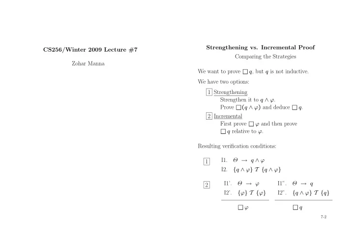
0 0 ( q ∧ ϕ ) and deduce 0 Strengthening vs. Incremental Proof CS256/Winter 2009 Lecture #7 0 Comparing the Strategies Zohar Manna 0 We want to prove q , but q is not inductive. We have two options: 1 Strengthening Strengthen it to q ∧ ϕ . Prove q . 2 Incremental First prove ϕ and then prove q relative to ϕ . 0 0 Resulting verification conditions: I1. Θ → q ∧ ϕ 1 I2. { q ∧ ϕ } T { q ∧ ϕ } I1’. Θ → ϕ I1”. Θ → q 2 I2’. { ϕ } T { ϕ } I2”. { q ∧ ϕ } T { q } ϕ q 7-2

Strengthening vs. Incremental Proof (Con’t) Strengthening vs. Incremental Proof (Con’t) Example: • 1 is strictly more powerful than 2 . 2 implies 1 since local x : integer where x = 1   ρ τ ∧ ϕ → ϕ ′ ℓ 0 : loop forever do � � � �� �   ℓ 1 : x := x + 1 I2’   → [ ρ τ ∧ q ∧ ϕ → q ′ ∧ ϕ ′   ]     ρ τ ∧ q ∧ ϕ → q ′ � �� �   I2   � �� � Show q 1 : at − ℓ 0 → x > 0 I2” q 2 : at − ℓ 1 → x > 0 • In practice, 2 is often more useful than 1 • both are P -valid – allows breaking down the proof in more manage- able pieces • neither of them is inductive – smaller verification conditions • but q 1 ∧ q 2 is inductive! – more intuitive 7-3 7-4

q Θ → χ i ) and so q 0 0 q q Θ → ϕ q ( Combining the Strategies Combining the Strategies (Con’t) q Θ → ϕ Rule inc-inv : (incremental invariance) Note that Θ must be stronger than all the χ i ’s (i.e., q ” and “ P q ”. P q For assertions q , ϕ , χ 1 ,. . . , χ k   I0. P χ 1 , . . . , χ k k �  ∧ Θ → ϕ q 0 iff P χ i P  k i =1 � I1. χ i ) ∧ ϕ → q P i =1 I2. P From now on, we usually omit “ P k � � � I3. P ( χ i ) ∧ ϕ T { ϕ } i =1 P q If ϕ satisfies I2 and I3, we say that “ ϕ is inductive relative to χ 1 , . . . χ k ” 7-5 7-6

Finding Inductive Assertions Detecting Trivial Verification Conditions Two methods: { ϕ } T { ϕ } – Don’t check every τ ∈ T . 1. Bottom-up: • Ignore { ϕ } τ I { ϕ } – always true • based on the program text only • Ignore { ϕ } τ { ϕ } • algorithmic if τ does not modify any variable in ϕ • guaranteed to produce an inductive invariant • For { ϕ } τ { ϕ } where ϕ : p → q 2. Top-down: → p ′ → q ′ ρ τ ∧ p → q � �� � � �� � ϕ ϕ ′ • guided by the property we want to prove Consider only τ ’s that • heuristic validate p or falsify q • not guaranteed to produce an inductive invariant 7-7 7-8

Finding Inductive Assertions Bottom-Up Approach (Con’t) Bottom-Up Approach • single variable assertions • Transition-validated assertions: y = 1 ℓ 1 : [ while c do S ]; ℓ 2 : at − ℓ 2 → ¬ c   loop forever do . . .     y ≥ 0   if no statement parallel to ℓ 2 can request y         modify variables in c   . . .       release y ℓ 1 : y := e ; ℓ 2 : at − ℓ 2 → y = e s = 1 if no statement parallel to ℓ 2 can modify y . . . . . .     s = 1 ∨ s = 2 or variables occurring in e s := 1  || s := 2    and if y does not occur in e . . . . . . . where no other statement modifies s 7-9 7-10

Example: Program square-root Program square-root Fig. 1.11 at − ℓ 2 → z 2 ≤ x < ( z + 1) 2 in x : integer where x ≥ 0 local u, w : integer where u = 1 , w = 1 out z : integer where z = 0 Intuitive argument: ℓ 0 : while w ≤ x do z = 0 , 1 , . . . , n ℓ 1 : ( z, u, w ) := ( z + 1 , u + 2 , w + u + 2) u = 1 , 3 , . . . , 2 n + 1 ℓ 2 : = ( z + 1) 2 w = 1 + 3 + . . . + (2 n +1) � �� � ( n +1) 2 ρ ℓ 0 : move ( ℓ 0 , ℓ 1 ) ∧ w ≤ x ∨ first time w > x � �� � ρ t ℓ 0 x < ( z + 1) 2 move ( ℓ 0 , ℓ 2 ) ∧ w > x � �� � ρ f last time w ≤ x ℓ 0 z 2 ≤ x ρ ℓ 1 : move ( ℓ 1 , ℓ 0 ) ∧ Thus at ℓ 2 : z ′ = z + 1 ∧ u ′ = u + 2 z 2 ≤ x < ( z + 1) 2 ∧ w ′ = w + u + 2 7-11 7-12

ψ 2 : at − ℓ 2 → x < ( z + 1) 2 Find • Step 2  w 0 = 1  � z 0 = 0   u n − 1   � �� � z n = z n − 1 + 1 for n > 0 w n = w n − 1 + ( 2( n − 1) + 1) + 2     = w n − 1 + (2 n + 1) for n ≥ 0  � u 0 = 1 n � (2 k + 1) = ( n + 1) 2 u n = u n − 1 + 2 for n > 0 w n = for n ≥ 0 k =0 w n = ( z n + 1) 2 for n ≥ 0 � w 0 = 1 w n = w n − 1 + u n − 1 + 2 for n > 0 ϕ 2 : w = ( z + 1) 2 • Step3 • Step 1 at − ℓ 2 → x < w � z n = n for n ≥ 0 ⇒ u n = 2 z n + 1 for n ≥ 0 for n ≥ 0 u n = 2 n + 1 Therefore ψ 2 : at − ℓ 2 → x < ( z + 1) 2 ϕ 1 : u = 2 z + 1 7-13 7-14

Construction of Linear Invariants Definition: A linear invariant is of the form a limited class of invariants that can be constructed algorithmically r � � a i · y i + b ℓ · at − ℓ = K i =1 ℓ ∈L Definition: integer variable y is linear in P if � �� � � �� � � �� � constant body compensation y ′ = y + c expression for every ρ τ for some integer constant c . where a i , b ℓ , K – integer constants. Example: semaphore variables are linear L – set of all locations in P y ′ = y + 1 y ′ = y − 1 y ′ = y y 1 , ..., y r – all linear variables in P � �� � � �� � � �� � request release otherwise 7-15 7-16

Example: Program double Assumption Program ℓ 1 0 : S 1 � . . . � ℓ i 0 : S i � . . . � ℓ m 0 : S m local y : integer where y = 0 • no nested parallel statements. Therefore, all move � ℓ 0 : y := y + 1 � � m 0 : y := y + 1 � expressions in all ρ τ are of the form move ( ℓ i , ℓ j ) ℓ 1 : m 1 : • all linear variables y i have a single initial value y 0 i linear variable: y • every transition τ enabled on some P -accessible state linear invariant: Increments y + at − ℓ 0 + at − m 0 = 2 if ρ τ → y ′ = y + c • ∆ ( y, τ ) = c therefore ρ τ → y ′ = y + ∆ ( y, τ ) How are linear invariants constructed?  1 if ℓ = ℓ j  Our procedure guarantees that the generated assertions  • ∆ ( at − ℓ, τ ) = − 1 if ℓ = ℓ i are P -invariants!  0 otherwise  if ρ τ → move ( ℓ i , ℓ j ) therefore ρ τ → at ′ − ℓ = at − ℓ + ∆ ( at − ℓ, τ ) 7-17 7-18

Equations (Con’d) Equations (T) the assertion has to be preserved by all transitions Construct (we want it to be inductive): r   � � r ϕ : a i · y i + b ℓ · at − ℓ = K � � a i · y i + b ℓ · at − ℓ = K ∧ ρ τ   i =1 ℓ ∈L i =1 ℓ ∈L � �� � ϕ We obtain the values of the coefficients from a set of equa-   r � � a i · y ′ b ℓ · at ′ tions as follows: → i + − ℓ = K   i =1 ℓ ∈L � �� � ϕ ′ (I) The invariant has to hold at the first state of every computation or r y i = y 0 implies i ( i = 1 . . . r ) Θ � � a i · ( y ′ b ℓ · ( at ′ ρ τ → i − y i ) + − ℓ − at − ℓ ) = 0 and π = { ℓ 1 0 , . . . , ℓ m 0 } i =1 ℓ ∈L resulting in the set of equations and so we get r � � a i · ∆ ( y i , τ ) + b ℓ · ∆ ( at − ℓ, τ ) = 0 r � a i · y 0 + ( b ℓ 1 0 + · · · + b ℓ m 0 ) = K i =1 ℓ ∈L i i =1 for every transition τ ∈ T 7-19 7-20

Example: Program double Example: Program double (Con’d) local y : integer where y = 0 � ℓ 0 : y := y + 1 � � m 0 : y := y + 1 � Possible solutions (basis for all solutions) ℓ 1 : m 1 : a b ℓ 0 b ℓ 1 b m 0 b m 1 K S 1 0 1 1 0 0 1 S 2 0 0 0 1 1 1 linear invariant: ϕ : a · y + b ℓ 0 · at − ℓ 0 + b ℓ 1 · at − ℓ 1 + S 3 1 1 0 1 0 2 b m 0 · at − m 0 + b m 1 · at − m 1 = K Corresponding invariants ( I ) a · 0 + b ℓ 0 + b m 0 = K (initial value of y is 0 ) (control invariant) ϕ 1 : at − ℓ 0 + at − ℓ 1 = 1 ϕ 2 : at − m 0 + at − m 1 = 1 (control invariant) (for ℓ 0 ) ( T ) a · 1 − b ℓ 0 + b ℓ 1 = 0 a · 1 − b m 0 + b m 1 = 0 (for m 0 ) ϕ 3 : y + at − ℓ 0 + at − m 0 = 2 7-21 7-22

Linear Invariants for Cyclic Programs Phase 1: Bodies For cycle ℓ 1 , ℓ 2 , . . . , ℓ k 0 : S 1 � . . . � ℓ j Program ℓ 1 0 : S j � . . . � ℓ m 0 : S m � �� � C where S j is of the form r ℓ j 0 : loop forever do ℓ j 1 , ℓ j 2 , . . . , ℓ j � a i · ∆ ( y i , τ ℓ 1 ) − b ℓ 1 + b ℓ 2 = 0 k � �� � i =1 cycle C r � a i · ∆ ( y i , τ ℓ 2 ) − b ℓ 2 + b ℓ 3 = 0 i =1 . . Define . r � ∆ ( y, C ) = ∆ ( y, τ 1 ) + · · · + ∆ ( y, τ k ) a i · ∆ ( y i , τ ℓ k ) + b ℓ 1 − b ℓ k = 0 i =1 For these programs construction of the linear invariants can be done in three phases: r � a i · ( ∆ ( y i , τ ℓ 1 ) + . . . + ∆ ( y i , τ ℓ k )) = 0 1. Compute a i ’s i =1 2. Compute b ℓ ’s 3. Compute K Thus, r � a i · ∆ ( y i , C ) = 0 i =1 7-23 7-24