[PDF] - Rolling CR-manifolds Setsuo TANIGUCHI Faculty of Arts and Science, PDF Document

SLIDE 1

Rolling CR-manifolds

Setsuo TANIGUCHI

Faculty of Arts and Science, Kyushu University

November 9, 2015

S. Taniguchi (Kyushu Univ)

Rolling CR-manifolds November 9, 2015 1 / 16 Introduction

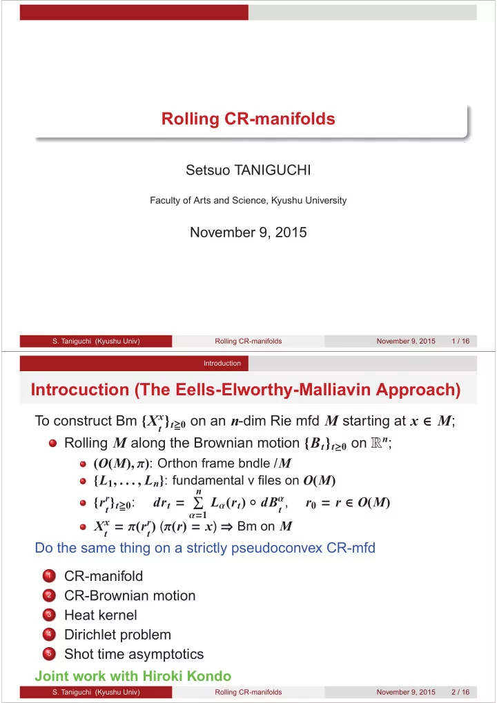
Introcuction (The Eells-Elworthy-Malliavin Approach)

To construct Bm {Xx

t }t≧0 on an n-dim Rie mfd M starting at x ∈ M;

Rolling M along the Brownian motion {Bt}t≥0 on Rn;

(O(M), π): Orthon frame bndle /M {L1, . . . , Ln}: fundamental v files on O(M) {rr

t}t≧0:

drt =

n

α=1

Lα(rt) ◦ dBα

t ,

r0 = r ∈ O(M) Xx

t = π(rr t) (π(r) = x) ⇒ Bm on M

Do the same thing on a strictly pseudoconvex CR-mfd

1

CR-manifold

2

CR-Brownian motion

3

Heat kernel

4

Dirichlet problem

5

Shot time asymptotics Joint work with Hiroki Kondo

S. Taniguchi (Kyushu Univ)

Rolling CR-manifolds November 9, 2015 2 / 16

SLIDE 2

CR-manifold

Strongly pseudoconvex CR-mfd

M is said to be a (2n + 1)-dim CR-mfd iff

1

real (2n + 1)-dimensional oriented C∞-mfd

2

∃ complex n-dim subbundle T1,0 of the complexified tangent

bundle CTM s.t. T1,0 ∩ T0,1 = {0}, where T0,1 = T1,0

3

Frobenius cond is fulfilled: [T1,0, T1,0] ⊂ T1,0

∃ 1-form θ 0 on M s.t. θ(H) = {0}

(H := Re(T1,0 ⊕ T0,1)) The Levi form Lθ is defined by

Lθ(Z, W) = −idθ(Z, W) (Z, W ∈ Γ∞(T1,0 ⊕ T0,1)),

where Γ∞(T1,0) is the totality of C∞-sections to T1,0.

M is strongly pseudoconvex iff the Levi form is strictly positive.

(Assumed here after)

S. Taniguchi (Kyushu Univ)

Rolling CR-manifolds November 9, 2015 3 / 16 CR-manifold

Examples

⋄ Real submfd of complex mfd N: complex mfd of (complex) dim n + 1 M: real 2n + 1-dim submfd of N T1,0 = T1,0N ∩ CTM,

where T1,0N is the hol tangent bdl/N

⋄ Hn = Cn × R: Heisenberg gr (z, t) · (w, s) = (z + w, s + t + 2Imz, w) Zα =

∂ ∂zα + iz α ∂ ∂t

T1,0 = spanC{Z1, . . . , Zn} θ = dt + i

n

α=1

zαdz

α − z αdzα

dθ = 2i

n

α=1 dzα ∧ dz

α

Lθ(Zα, Zβ) = δαβ

S. Taniguchi (Kyushu Univ)

Rolling CR-manifolds November 9, 2015 4 / 16

SLIDE 3

CR-manifold

Kohn-Rossi Laplacian

ψ := θ ∧ (dθ)n; vol form L∗

θ :=the dual on H∗ of Lθ on H = Re(T1,0 ⊕ T0,1).

u, vθ =

M

uvψ, ω, ηθ =

M

L∗

θ(ω, η)ψ

(u, v ∈ C∞

0 (M), ω, η ∈ Γ(H∗)).

db := r0 ◦ d, ∂b := r1 ◦ d,

where r0 : T∗M → H∗, r1 : T∗M → T∗

0,1: projections

Sublaplacian ∆b := db

∗db, K-R Laplacian b := ∂b ∗ ∂b:

∆bu, vθ = dbu, dbvθ, bu, vθ = ∂bu, ∂bvθ. ∃1T: v field transversal to H with T⌋dθ = 0 and T⌋θ = 1.

Then b = ∆b + inT.

S. Taniguchi (Kyushu Univ)

Rolling CR-manifolds November 9, 2015 5 / 16 CR-manifold

Tanaka-Webster connection

J : H → H; the complex structure; J = i on T1,0, = −i on T0,1 gθ: the Webster metric; for X, Y ∈ H gθ(X, Y) = dθ(X, JY), gθ(X, T) = 0, & gθ(T, T) = 1

Tanaka-Webster connection: ∃! lin conn ∇

∇X(Γ∞(H)) ⊂ Γ∞(H) (∀X ∈ Γ∞(TM)), ∇J = 0, ∇gθ = 0 T∇(Z, W) = 0, T∇(Z, V) = 2iLθ(Z, V)T

for Z, W ∈ Γ∞(T1,0), V ∈ Γ∞(T0,1) where T∇(Z, W) = ∇ZW − ∇WZ − [Z, W]

T∇(T, JX) + J(T∇(T, X)) = 0 for X ∈ Γ∞(TM)

n := {1, . . . , n} & n := {0, 1, . . . , n, 1, . . . , n},

where α; Zα := Zα For a local orthon frame {Zα}α∈n (Zα ∈ Γ∞(U; T1,0)),

∇Z AZB =

C∈ n ΓC ABZC, A, B ∈

n

(Z0 = T)

ΓC

AB = 0 if (B, C) {(β, γ), (β, γ)|β, γ ∈ n}

S. Taniguchi (Kyushu Univ)

Rolling CR-manifolds November 9, 2015 6 / 16

SLIDE 4

CR-manifold

Fundamental vector fields

p : [a, b] → T1,0 is parallel along p : [a, b] → M

iff

p(t) ∈ (T1,0)p(t) and ∇ ˙

p

p = 0 U(T1,0) := ∐x∈M{r : Cn → (T1,0)x : isometric}, π(r) = x U(n)-principal bundle

p : [a, b] → U(T1,0) is a horizontal lift of p : [a, b] → M

iff π(

p) = p, p(t)ξ is pararel along p (∀ξ ∈ Cn)

For v ∈ TxM, η ∈ Tr(U(T1,0)) (π(r) = x) is a holizontal lift of v if ∃

p, a holizontal lift of p s.t. p(0) = r, ˙

p(0) = η, π∗η = v.

For v ∈ TxM and r ∈ U(T1,0) with π(r) = x,

∃!ηr(v) ∈ Tr(U(T1,0)); holizontal lift of v (Lα)r := ηr(reα), α ∈ n; v fields on U(T1,0)

where {eα}α∈n is the standard basis of Cn

S. Taniguchi (Kyushu Univ)

Rolling CR-manifolds November 9, 2015 7 / 16 CR-manifold

Local expression

For a local orhon frame {Zα}α∈n of T1,0, set {eβ

α(r)} ∈ Cn×n by r(eα) = β∈n eβ α(r)(Zβ)π(r).

Lα =

β∈n

eβ

αZβ −

β,γ,δ,ε∈n

Γγ

βδeδ εeβ α

∂ ∂eγ

ε

−

β,γ,δ,ε∈n

Γγ

βδeδ εeβ α

∂ ∂eγ

ε

S. Taniguchi (Kyushu Univ)

Rolling CR-manifolds November 9, 2015 8 / 16

SLIDE 5

CR-Brownian motion

{Bt = (B1

t, . . . , Bn t )}t≧0: Cn-valud continuous martingale with

Bα, Bβt = 0 & Bα, Bβt = δαβt. {rr

t}t≧0: the unique sol to the SDE on U(T1,0):

drt =

n

α=1{Lα(rt) ◦ dBα

t + Lα(rt) ◦ dBα t },

r0 = r ∈ U(T1,0) Qr:=the distribution of {rr

t}t≧0 on C([0, ∞); U(T1,0)).

Px := Qr ◦ π−1 (r ∈ π−1(x))

(π : U(T1,0) → M: proj) Rem: Qr ◦ π−1 = Qr′ ◦ π−1 if π(r) = π(r′), since r(t, ur, uB) = r(t, r, B) (u ∈ U(n)). Let Xt : C([0, ∞); M) → M be the coord pr.

{({Xt}t≧0, Px), x ∈ M} is the diffusion generated by − 1

2∆b

(CR-Brownian motion)

∵ − 1

2∆b = 1 2 n

α=1

LαLα + LαLα

C∞(M)
S. Taniguchi (Kyushu Univ)

Rolling CR-manifolds November 9, 2015 9 / 16 Heat kernel

Partial hyperellipticity

Let P, N be C∞-mfds, φ : P → N be C∞,

A0, . . . , An be C∞-v fields on P. Xt be the sol to the SDE on P: dXt =

n

α=1 Aα(Xt) ◦ dBα

t + A0(Xt)dt

Yt := φ(Xt)

Theorem 0 (T83) Assume that

(φ∗)p(Lp) = Tφ(p)N (∀p ∈ P),

where

L =

[Ai1, . . . , [Aik, A j] . . . ]
1 ≤ j ≤ n, 0 ≤ iℓ ≤ n, k ∈ Z≥0
.

Then Yt admits a C∞-density function.

P = O(M), N = M ⇒ ∃ heat kernel for 1

2∆M

S. Taniguchi (Kyushu Univ)

Rolling CR-manifolds November 9, 2015 10 / 16

SLIDE 6

Heat kernel

Coming back to the CR-mfd; Let {Zα} be a local orthonormal frame for T1,0. Then

(π∗)Lα =

n

β=1

eβ

αZβ.

(π∗)[Lα, Lα] = −iT mod {Zβ, Zβ ; β = 1, . . . , n}.

Hence

spanR (π∗)rReLα, (π∗)rImLα, (π∗)r[ReLα, ImLα] : 1 ≤ α ≤ n = Tπ(r)M

(∀r ∈ U(T1,0)). Under a suitable non-explosion assumption (assumed hereafter), by Theorem 0, Theorem 1

∃p ∈ C∞((0, ∞) × M × M) s.t. Px(Xt ∈ dy) = p(t, x, y)ψ(dy).

S. Taniguchi (Kyushu Univ)

Rolling CR-manifolds November 9, 2015 11 / 16 Dirichlet problem

Dirichlet problem

Let G be a rel cpt conn open set in M with C3-bdry

τ′ = inf{t ≥ 0 : Xt G}.

For f ∈ C(∂G), define uf(x) := Ex[f(Xτ′)]. Theorem 2 (Probabilistically)

⋄ u f ∈ C(G) ⋄ uf, ∆bvθ = 0

(∀v ∈ C0(G)) & u f|∂G = f. Under local orthon frame {Zα},

−∆b =

n

α=1{Z2

α + Z2 α} + b,

[ReZα, ImZα] = 1

2T mod {ReZβ, ImZβ; 1 ≤ β ≤ n}

Corollary 3

uf ∈ C∞(G); u f is a classical sol to the Diriclet problem for ∆b

S. Taniguchi (Kyushu Univ)

Rolling CR-manifolds November 9, 2015 12 / 16

SLIDE 7

Dirichlet problem

Stroock-Varadhan (1972): It suffices to show (a) supx∈G Ex[τ′] < ∞ (b) Px(τ′ = 0) = 1 (∀x ∈ ∂G)

dXt =

2n

i=1 Vi(Xt) ◦ dbi

t + V0(Xt)dt,

where V2i =

√ 2 ReZi, V2i−1 = √ 2 ImZi & V0 = −b

(a) Controlability + a standard argument (b) Stroock-T (1986):

Γ = {x ∈ ∂G | Px(τ′ = 0) = 1} ΨL =

x ∈ ∂G
Viφ = 0 (i < L),

i=L(Viφ)2(x) 0

,

where, for i = (i1, . . . , ik) ∈ {0, 1, . . . , 2n}k,

Vi = Vi1 ◦ · · · ◦ Vik and i = k + #{ j | ij = 0} L; odd ⇒ ΨL ⊂ Γ L = 2; x ∈ ΨL is in Γ if either

(i) M := (ViVjφ(x))1≤i,j≤n is not symmetric (ii) M is symmetric but admits at least 1 negative ev (iii) V0φ(x) < 0

S. Taniguchi (Kyushu Univ)

Rolling CR-manifolds November 9, 2015 13 / 16 Short time asymptotics

Short time asymptotics

Theorem 4 It holds that

p(t, x, x) ∼ 1 tn+1

∞

k=0

Ck(x)t k as t ↓ 0.

Furthermore C0(x) = C0 =

1 (4π)n+1n!

R
2τ

sinh(2τ) ndτ

1

Localization around x ∈ M:

{Zα}: a loc orthonormal frame of T1,0 on a rel cpt coord nbd U V: an open rel cpt subset of U with x ∈ V. Xα := √ 2 ReZα, Xn+α := √ 2 ImZα, α = 1, . . . , n. {(Xt, ˜ Py) : y ∈ U}: the diffusion generated by

1 2

2n

k=1 X2 k − 1 2

n

α,β=1

Γα

ββ

Zα + Γα

ββ

Zα

˜

p(t, x, y): a density function of ˜ Py with respect to ψ

S. Taniguchi (Kyushu Univ)

Rolling CR-manifolds November 9, 2015 14 / 16

SLIDE 8

Short time asymptotics 2

p(t, x, x) ∼ ˜ p(t, x, x)

3

We do not rely on Stochastic Taylor expansion, but employ a purturbation argument:

Folland-Stein (1974):

∃ a coord sys u = (u0, u1, . . . , u2n) around x s.t. u(x) = 0 & X j = ∂ ∂uj + 2un+ j ∂ ∂u0 +

2n

k=1

O j,1 ∂ ∂uk + Oj,2 ∂ ∂u0 , Xn+ j = ∂ ∂un+j − 2uj ∂ ∂u0 +

2n

k=1

On+ j,1 ∂ ∂uk + On+j,2 ∂ ∂u0 , T = ∂ ∂u0 +

2n

k=1

O2n+1,1 ∂ ∂uk ,

where O∗,i = O|u0|1/2 + 2n

1 |uk|i as (u0, . . . , u2n) → 0.

S. Taniguchi (Kyushu Univ)

Rolling CR-manifolds November 9, 2015 15 / 16 Short time asymptotics