Road Map When Costs and Probabilities are Both Unknown Problem - - PowerPoint PPT Presentation

Learning and Making Decisions When Costs and Probabilities are Both Unknown

Bianca Zadrozny and Charles Elkan

Presenter: Aurora

Road Map

• Problem and Challenge Formulation
• Preliminary Knowledge
• Cost-Sensitive Learning Methods
• Probability Estimation
• Donation Amount Estimation
• Experiments
• Contributions

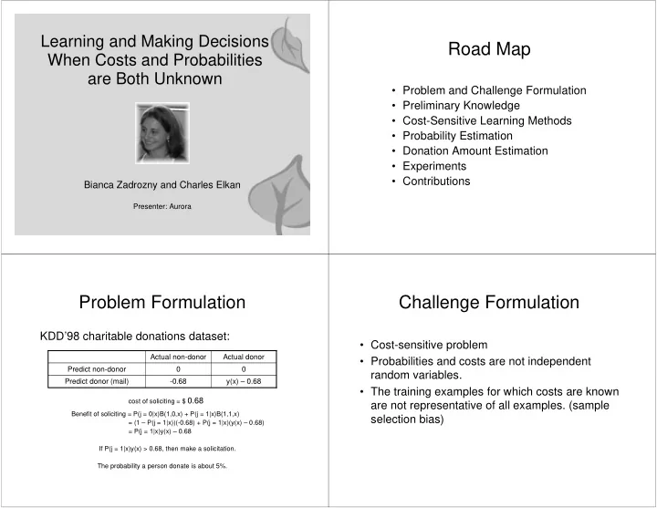
Problem Formulation

KDD’98 charitable donations dataset:

cost of soliciting = $ 0.68 Benefit of soliciting = P(j = 0|x)B(1,0,x) + P(j = 1|x)B(1,1,x) = (1 – P(j = 1|x))(-0.68) + P(j = 1|x)(y(x) – 0.68) = P(j = 1|x)y(x) – 0.68 If P(j = 1|x)y(x) > 0.68, then make a solicitation. The probability a person donate is about 5%.

y(x) – 0.68

• 0.68

Predict donor (mail) Predict non-donor Actual donor Actual non-donor

Challenge Formulation

• Cost-sensitive problem
• Probabilities and costs are not independent

random variables.

• The training examples for which costs are known

are not representative of all examples. (sample selection bias)

Preliminary Knowledge

Bias vs. Variance

• Bias: This quantity measures how closely the learning algorithm’s average

guess (over all possible training sets of the given training set size) matches the target.

• Variance: This quantity measures how much the learning algorithm’s

guess fluctuates for the different training sets of the given size.

Stable vs. Unstable Classifier

Unstable Classifier: Small perturbations in the training set or in construction may result in large changes in the constructed predictor.

• Unstable Classifiers: Decision Tree, ANN

Characteristically have high variance and low bias.

• Stable Classifiers: Naïve Bayes, KNN

Have low variance, but can have high bias.

Preliminary Knowledge

Bagging

Bagging votes classifiers generated by different bootstrap samples. A bootstrap sample is generated by uniformly sampling m instances from the training set with

• replacement. T bootstrap samples B1, B2, …, BT are

generated and a classifier Ci is built from each Bi. A final classifier C is built from C1, C2, …, CT by voting.

Bagging can reduce the variance of unstable classifiers.

Cost-Sensitive Learning Methods

• --- compare with previous work

ÿ P(j|x) C(i,j,x)

• MetaCost

– Train ÿ P(j|x) C(i,j,x) estimator for each example. – Assumption: costs are known in advance and are the same for all examples. – Use bagging to estimate probabilities.

• Direct Cost-Sensitive Decision-Making

– Train P(j|x) estimator and C(i,j,x) estimator for each example. – Cost is unknown for test data and example-dependent. – Use decision tree to estimate probabilities.

Why bagging is not suitable for estimating conditional probability?

1. Bagging gives voting estimates that measure the stability of the classifier learning method at an example, not the actual class conditional probability

• f the example.

How does bagging in MetaCost work? Eg: Among n sub-classifiers, k of them give class label 1 for x, then P(j = 1|x) = k / n. My solution: Use the average of the probabilities over all sub-classifiers as the final probability.

2. Bagging can reduce the variance of the final classifier by combining several classifiers, but can not remove the bias of each sub-classifier.

Probability Estimation

• --- Obtain calibrated probability estimation from

decision tree and Naïve Bayesian

• Decision Tree

Unstable – Smoothing – Curtailment

• Naïve Bayesian

Stable – Binning

• Averaging Probability Estimators

Raw Decision Tree Conditional Probability Estimation

Assign p = k/n as the conditional probability for each example that is assigned to a decision tree leaf that contains k positive training examples and n total training examples.

Deficiencies of Decision Tree

• High bias: Decision tree growing methods try to make leaves

homogeneous, so observed frequencies are systematically shifted towards zero and one.

Smoothing

• High variance: When the number of training examples associated with a

leaf is small, observed frequencies are not statistically reliable.

Curtailment,

(Not pruning, because pruning is based on error rate minimization, not cost minimization.)

Smoothing

Base rate: b = 0.05 m = 10 m = 100 As m increases, probabilities are shifted more towards the base rate. One way to improve the probability estimation of decision tree is to make these estimation less extreme. replace by

Curtailment

If the parent of a small leaf contains enough examples to induce a statistically reliable probability estimate, then assigning this estimate to a test example associated with the leaf may be more accurate then assigning it a combination of the base rate and the observed leaf frequency.

Deficiency of Naïve Bayes

Assumption: Attributes of examples are independent. Actually attributes tend to be correlated, so scores are typically too extreme: for n(x) near 0, n(x) < P(j = 1|x) (positively correlated) for n(x) near 1, n(x) > P(j = 1|x) (negatively correlated) Solution: Binning The probability that x belongs to class j is the fraction of training examples in the bin that actually belong to j, which is represented with the blue star.

Averaging Probability Estimators

Intuition: If the classifiers are partially uncorrelated, variance can be reduced by averaging combination.

is the variance of each original classifier. is the correlation factor N is the number of classifiers

Donation Amount Estimation

• Least-Squares Multiple Linear Regression

Linear

• Variance of Heckman’s Method
• -- Sample Selection Bias

Non-Linear

Least-Squares Multiple Linear Regression

Two attributes:

Lastgift: dollar amount of the most recent donation Ampergift: average donation amount in responses to

the last 22 promotions

Sample Selection Bias

Definition: The training examples used to learn a model are drawn from a different probability distribution than the examples to which the model is applied. Situation: The donation amounts estimator is trained based on examples of people who actually donate, but this estimator must then be applied to a different population --- both donors and non-donors.

• Heckkman’s solution:

1. Learn a probit linear model to estimate conditional probabilities P(j = 1|x). 2. Estimate y(x) by linear regression using only the training examples x for which j(x) = 1, but including for each x a transformation of the estimated value of P(j = 1|x).

• Bianca’s solution:

1. Instead of using a linear estimator for P(j = 1|x), she uses non- linear estimator decision tree or naïve Bayes classifier. 2. Use a non-linear learning method to obtain an estimator for y(x). Three attributes: Lastgift, Ampergift, P(j = 1|x)

Experiment

The performance of direct cost-sensitive decision- making is better than MetaCost. While both can be improved by any technique proposed for probability estimation.

direct cost-sensitive decision- making MetaCost

Contributions

• Provide a cost-sensitive learning method: direct cost-

sensitive decision-making, which is better than the previous method MetaCost.

• Provide several techniques to improve the

performance of probability estimator.

• Provide solution to the problem of costs being

example-dependent and unknown in general.

• Provide solution to the problem of sample selection

bias.