Representing metabolic networks In the following we assume that we - - PowerPoint PPT Presentation

Representing metabolic networks

◮ In the following we assume

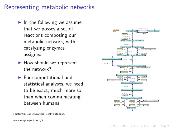
that we posses a set of reactions composing our metabolic network, with catalyzing enzymes assigned

◮ How should we represent

the network?

◮ For computational and

statistical analyses, we need to be exact, much more so than when communicating between humans

(picture:E.Coli glycolysis, EMP database, www.empproject.com/)

Levels of abstraction

◮ Everything relevant should be included in our representation ◮ What is relevant depends on the questions that we want to

solve

◮ There are several levels of abstraction to choose from

• 1. Graph representations: Connectivity of reactions/metabolites,

structure of the metabolic network

• 2. Stoichiometric (reaction equation) representation: capabilities
• f the network, flow analysis, steady-state analyses
• 3. Kinetic models: dynamic behaviour under changing conditions

Representing metabolic networks as graphs

For structural analysis of metabolic networks, the most frequently encountered representations are:

◮ Enzyme interaction network ◮ Reaction graph ◮ Substrate graph

We will also look briefly at

◮ Atom-level representations ◮ Boolean circuits (AND-OR graphs)

Example reaction List

◮ A set of reactions implementing a part of pentose-phosphate

pathway of E. Coli

◮ Enzyme catalyzing the reaction annoted over the arrow symbol

R1: β-D-glucose 6-phosphate (βG6P) + NADP+ zwf ⇒ 6-phosphoglucono-lactone (6PGL) + NADPH R2: 6-phosphoglucono δ-lactone + H2O

pgl

⇒ 6-phosphogluconate (6PG) R3: 6-phosphogluconate + 1 NADP+ gnd ⇒ ribulose 5-phosphate (R5P) + NADPH R4: ribulose 5-phosphate (R5P)

rpe

⇒ xylulose 5-phosphate (X5P) R5: α-D-glucose 6-phosphate(αG6P)

gpi

⇔ βG6P R6: α-D-glucose 6-phosphate(αG6P)

gpi

⇔ β-D-Fructose-6-phosphate (βF6P) R7: β-D-glucose 6-phosphate(αG6P)

gpi

⇔ βF6P

Enzyme interaction networks

◮ Enzymes as nodes ◮ Link between two enzymes

if they catalyze reactions that have common metabolites

◮ A special kind of

protein-protein interaction network

Enzyme interaction network construction

◮ In our pathway, we have 5

enzymes catalyzing a total

• f 7 reactions

R1: βG6P + NADP+ zwf ⇒ 6PGL + NADPH R2: 6PGL + H2O

pgl

⇒ 6PG R3: 6PG + NADP+ gnd ⇒ R5P + NADPH R4: R5P

rpe

⇒ X5P R5: αG6P

gpi

⇔ βG6P R6: αG6P

gpi

⇔ βF6P R7: βG6P

gpi

⇔ βF6P

rpe gnd pgl gpi zwf

Enzyme interaction network construction

◮ We take each pair of

enzymes in turn

◮ Draw and edge between if

they share metabolites

◮ (gpi,zwf) — βG6P

R1: βG6P + NADP+ zwf ⇒ 6PGL + NADPH R2: 6PGL + H2O

pgl

⇒ 6PG R3: 6PG + NADP+ gnd ⇒ R5P + NADPH R4: R5P

rpe

⇒ X5P R5: αG6P

gpi

⇔ βG6P R6: αG6P

gpi

⇔ βF6P R7: βG6P

gpi

⇔ βF6P rpe gnd pgl gpi zwf

Enzyme interaction network construction

◮ We take each pair of

enzymes in turn

◮ Draw and edge between if

they share metabolites

◮ (zwf, pgl) — 6PGL

R1: βG6P + NADP+ zwf ⇒ 6PGL + NADPH R2: 6PGL + H2O

pgl

⇒ 6PG R3: 6PG + NADP+ gnd ⇒ R5P + NADPH R4: R5P

rpe

⇒ X5P R5: αG6P

gpi

⇔ βG6P R6: αG6P

gpi

⇔ βF6P R7: βG6P

gpi

⇔ βF6P rpe gnd pgl gpi zwf

Enzyme interaction network construction

◮ (zwf, gnd) — NADP,

NADPH

◮ (zwf, rpe) — ∅

R1: βG6P + NADP+ zwf ⇒ 6PGL + NADPH R2: 6PGL + H2O

pgl

⇒ 6PG R3: 6PG + NADP+ gnd ⇒ R5P + NADPH R4: R5P

rpe

⇒ X5P R5: αG6P

gpi

⇔ βG6P R6: αG6P

gpi

⇔ βF6P R7: βG6P

gpi

⇔ βF6P rpe gnd pgl gpi zwf

Enzyme interaction network construction

◮ (pgl,gnd) — 6PG ◮ (gnd, rpe) — R5P

R1: βG6P + NADP+ zwf ⇒ 6PGL + NADPH R2: 6PGL + H2O

pgl

⇒ 6PG R3: 6PG + NADP+ gnd ⇒ R5P + NADPH R4: R5P

rpe

⇒ X5P R5: αG6P

gpi

⇔ βG6P R6: αG6P

gpi

⇔ βF6P R7: βG6P

gpi

⇔ βF6P rpe gnd pgl gpi zwf

Enzyme interaction network construction

◮ (zwf, gnd) — NADP,

NADPH

◮ (pgl,gnd) — 6PG ◮ (gnd, rpe) — R5P

R1: βG6P + NADP+ zwf ⇒ 6PGL + NADPH R2: 6PGL + H2O

pgl

⇒ 6PG R3: 6PG + NADP+ gnd ⇒ R5P + NADPH R4: R5P

rpe

⇒ X5P R5: αG6P

gpi

⇔ βG6P R6: αG6P

gpi

⇔ βF6P R7: βG6P

gpi

⇔ βF6P rpe gnd pgl gpi zwf

Reaction clumping in Enzyme networks

As each enzyme is represented once in the network reactions catalyzed by the same enzyme will be clumped together:

◮ For example, an alcohol dehydrogenase enzyme (ADH)

catalyzes a large group of reactions of the template: an alcohol + NAD+ <=> an aldehyde or ketone + NADH + H+

◮ Mandelonitrile lyase catalyzes a single reaction:

Mandelonitrile <=> Cyanide + Benzaldehyde

◮ The interaction between the two is very specific, only via

benzaldehyde, but this is not deducible from the enzyme network alone

Co-factor effects

◮ A group of ”currency

molecules” (ATP,ADP,NAD,NADH, NADP, NADPH) act as co-factors in many reactions

◮ The reactions that share

the co-factors may not

• therwise have anything in

common

◮ Sharing a co-factor induces

an arc between reactions.

◮ This can be misleading,

unless we are specifically interested in co-factors

zwf: G6P + NADP+ ⇒ 6PGL + NADPH gnd: 6PG + NADP+ ⇒ R5P + NADPH

rpe gnd pgl gpi zwf

Co-factor effects

◮ For example, the edge

(zwf,gnd) in our example network arises solely because of the co-factor molecules (NADP,NADPH)

◮ This fact cannot be

decuded from the enzyme network

◮ Chance to be mislead?

zwf: G6P + NADP+ ⇒ 6PGL + NADPH gnd: 6PG + NADP+ ⇒ R5P + NADPH

rpe gnd pgl gpi zwf

Reaction graph

A reaction graph removes the reaction clumping property of enzyme networks.

◮ Nodes correspond to reactions ◮ A connecting edge between two reaction nodes R1 and R2

denotes that they share a metabolite Difference to enzyme networks

◮ Each reaction catalyzed by an enzyme as a separate node ◮ A reaction is represented once, even if it has multiple

catalyzing enzymes

Reaction graph example

R1: βG6P + NADP+ zwf ⇒ 6PGL + NADPH R2: 6PGL + H2O

pgl

⇒ 6PG R3: 6PG + NADP+ gnd ⇒ R5P + NADPH R4: R5P

rpe

⇒ X5P R5: αG6P

gpi

⇔ βG6P R6: αG6P

gpi

⇔ βF6P R7: βG6P

gpi

⇔ βF6P

R1 R2 R4 R3 R5 R6 R7

Edge Supporting metabolites (R6,R7): βF6P (R6,R5): αG6P (R5,R7) βG6P (R7,R1): βG6P (R1,R2): 6PGL (R1, R3): NADP, NADPH (R2,R3): 6PG (R3, R4): R5P

Substrate graph

A dual representation to a reaction graph is a substrate graph.

◮ Nodes correspond to metabolites ◮ Connecting edge between two metabolites A and B denotes

that there is a reaction where both occur as substrates, both

• ccur as products or one as product and the other as substrate

◮ A reaction A + B ⇒ C + D is spread among a set of edges

{(A, C), (A, B), (A, D), (B, C), (B, D), (C, D)}

Substrate graph example

◮ Add and edge between all molecule pairs in R1 ◮ (G6P,NADPH), (G6P,6PGL), (G6P,NADP+),

(NADP+,NADPH), (NADP+, 6PGL), (6PGL, NADPH)

R1: βG6P + NADP+ zwf ⇒ 6PGL + NADPH R2: 6PGL + H2O

pgl

⇒ 6PG R3: 6PG + NADP+ gnd ⇒ R5P + NADPH R4: R5P

rpe

⇒ X5P R5: αG6P

gpi

⇔ βG6P R6: αG6P

gpi

⇔ βF6P R7: βG6P

gpi

⇔ βF6P

H O 2 + NADP F6P

β

G6P α G6P NADPH X5P R5P 6PG 6PGL

Substrate graph example

◮ Add and edge between all molecule pairs in R2 ◮ (6PGL,6PG), (6PGL,H2O), (6PG,H2O)

R1: βG6P + NADP+ zwf ⇒ 6PGL + NADPH R2: 6PGL + H2O

pgl

⇒ 6PG R3: 6PG + NADP+ gnd ⇒ R5P + NADPH R4: R5P

rpe

⇒ X5P R5: αG6P

gpi

⇔ βG6P R6: αG6P

gpi

⇔ βF6P R7: βG6P

gpi

⇔ βF6P

H O 2 G6P NADPH + X5P R5P 6PG 6PGL F6P G6P α β NADP

Substrate graph example

◮ Add and edge between all molecule pairs in R3 ◮ (6PG,NADP+),(6PG,R5P), (6PG,NADPH), (NADP+, R5P),

(R5P,NADPH)

R1: βG6P + NADP+ zwf ⇒ 6PGL + NADPH R2: 6PGL + H2O

pgl

⇒ 6PG R3: 6PG + NADP+ gnd ⇒ R5P + NADPH R4: R5P

rpe

⇒ X5P R5: αG6P

gpi

⇔ βG6P R6: αG6P

gpi

⇔ βF6P R7: βG6P

gpi

⇔ βF6P

H O 2 G6P NADPH + X5P R5P 6PG 6PGL F6P G6P α β NADP

Substrate graph example

R1: βG6P + NADP+ zwf ⇒ 6PGL + NADPH R2: 6PGL + H2O

pgl

⇒ 6PG R3: 6PG + NADP+ gnd ⇒ R5P + NADPH R4: R5P

rpe

⇒ X5P R5: αG6P

gpi

⇔ βG6P R6: αG6P

gpi

⇔ βF6P R7: βG6P

gpi

⇔ βF6P

H O 2 G6P NADPH NADP + X5P R5P 6PG 6PGL F6P G6P α β

Graph analyses of metabolism

Enzyme interaction networks, reaction graphs and substrate graph can all be analysed in similar graph concepts and algorithms We can compute basic statistics of the graphs:

◮ Connectivity of nodes: degree k(v) of node v; how many

edges are attached to each node.

◮ Path length between pairs of nodes ◮ Clustering coeefficient: how tightly connected the graph is

Clustering coefficient

◮ Clustering coefficient measures the

connectivity of graph around single nodes

◮ Informally: How close to a fully connected

graph are the neighbors of given node v, if we remove the node v and all edges adjacent to it

◮ In the example on the right, the clustering

coefficient of the blue node is given for three different neighborhoods

Clustering coefficient formally

Clustering coefficient C(v) for node v measures to what extent v is within a tight cluster

◮ Let G = (V , E) be a graph with nodes V and edges E ◮ Let N(v) be the set of nodes adjacent to v ◮ The clustering coefficient is the relative number of edges

between the nodes in N(v): C(v) = |{(v′, v′′) ∈ E|v′, v′′ ∈ N(v)}| Nmax , where Nmax = max{|N(v)|(|N(v)| − 1)/2, 1}

◮ Maximum C(v) = 1 occurs when N(v) is a fully connected

graph

◮ Clustering coefficient of the whole graph is the node average:

C(G) = 1/n

v(C(v)))

Clustering coefficient in our enzyme network

◮ N(gpi) = {zwf },

C(gpi) = 0

◮ N(zwf ) = {gpi, pgl, gnd},

C(zwf ) = |{(pgl,gnd)}|

3

= 1/3

◮ N(pgl) = {zwf , gnd},

C(pgl) = |{(zwf ,gnd)}|

1

= 1/1

◮ N(gnd) = {rpe, zwf , gnd},

C(gnd) = |{(zwf ,pgl)}|

3

= 1/3

◮ N(rpe) = {gnd},

C(rpe) = 0

◮ C(G) = 1/3

rpe gnd pgl gpi zwf

Comparison to graphs with known generating mechanism

One way to analyse our graphs is to compare the above statistics to graphs that we have generated ourself and thus know the generating mechanism. We will use the following comparison:

◮ Erd¨

• s-Renyi (ER) random graph

◮ Small-world graphs with preferential attachment

Erd¨

• s-Renyi random graph

◮ Well studied model for

random graphs proposed by Paul Erd¨

• s and Alfred

Renyi in 1959

◮ Generation of ER graph:

◮ Start with a network

with n nodes and no edges.

◮ Draw an edge between

each pair of nodes is with probability p.

Properties of ER graph

◮ ER graph of size n has on average

n

2

• p edges.

◮ Node degree distribution of is binomial

P(deg(v) = k) = n − 1 k

• pk(1 − p)n−1−k

◮ The connectivity of ER graph follows directly from the

quantities n and p:

◮ p < (1−ǫ) ln n

n

: graph will almost surely be non-connected

◮ p > (1+ǫ) ln n

n

: graph will almost surely be connected

◮ np < 1: graph will almost surely have no large connected

components, otherwise almost surely will have one

◮ Due to its mathematical elegance, ER model has been very

popular subject of study in graph theory

ER networks and biology

◮ It has been observed that the ER graph is not a good

explanation for the generating mechanism of many biological networks

◮ Prime symptom is that the node degree distribution of

biological networks does not fit to binomial distribution

◮ In particular, biological networks often have so called hubs,

nodes with very high connectivity

Preferential attachment

Preferential attachment (PA) is a mechanism that is proposed to generate many networks occurring in nature.

◮ Start with a small number n0 of nodes and no edges. ◮ Iterate the following:

◮ insert a new node v, ◮ draw m ≤ n0 edges from v to existing nodes vi with probability

p ∼

ki+1 P

j(kj+1)

When drawing new edges, nodes with many edges already are preferred over nodes with few or no edges.

◮ Hubs, i.e. highly connected nodes, will emerge from the

generating process

Degree distributions of ER and PA graphs

◮ P(k) - The probability of

encountering a node with degree k:

◮ Erd¨

• s-Renyi random graph:

P(k) ≈ n

k

• pk(1 − p)n−k.

◮ Distribution tightly peaked

around the average degree: low variance.

◮ Frequency of nodes with

very high degree is low.

Degree distributions of ER and PA graphs

◮ P(k) - The probability of

encountering a node with degree k:

◮ Preferential attachment:

P(k) ≈ k−γ.

◮ Frequency distribution is

scale-free: log P(k) and log k are linearly correlated.

◮ Distribution has a fat tail:

high variance and high number of nodes with high degree.

Degree distributions in metabolism (Wagner & Fell, 2000)

Degree distributions of substrate and reaction graphs

Degree distributions in metabolism (Wagner & Fell, 2000)

◮ Substrate graph

shows a fat-tailed distribution

◮ consistent with a

network generated via preferential attachment.

Small-world graphs

Graphs fulfilling the following two criteria are called small-world graphs

◮ Small average shortest path length between two nodes

◮ The same level as ER graphs, lower than many regular graphs: ◮ Shortcuts accross the graphs go via hubs

◮ High clustering coefficient compared to ER graph: the

neighbors of nodes are more often linked than in ER graphs. Graphs generated with preferential attachment are small-world graphs.

Small-world graphs

Graphs fulfilling the following two criteria are called small-world graphs

◮ Small average shortest path length between two nodes

◮ The same level as ER graphs, lower than many regular graphs: ◮ Shortcuts accross the graphs go via hubs

◮ High clustering coefficient compared to ER graph: the

neighbors of nodes are more often linked than in ER graphs. Graphs generated with preferential attachment are small-world graphs. However, small-world graphs can be generated with other mechanisms as well...

Metabolic graphs as small worlds

◮ Path lengths in

reaction and substrate graphs are about the same as Erd¨

• s-Renyi

random graph with the same average connectivity

◮ Clustering coefficients

are much larger than in ER graphs

◮ The graphs resemble

small-world graphs

Pitfalls in substrate graph analysis: co-factors

◮ Path length in substrate graphs may not be biologically

relevant

◮ Shortest paths between metabolites in otherwise distant parts

• f metabolism tend to go through co-factor metabolites

(NADP, NAPH, ATP, ADP).

◮ However, transfer of atoms occurs only between the co-factors

Pitfalls in substrate graph analysis: co-factors

Quick remedy used in most studies:

◮ Remove co-factors from the graph ◮ But sometimes it is difficult to decide which ones should be

removed and which ones to leave.

Atom-level representation

◮ Better solution is to trace the atoms accross pathways ◮ An acceptable path needs to involve transfer of atoms from

source to target.

◮ Spurious pathways caused by the co-factor problem are

filtered out

◮ This paradigm is used by Arita in his ARM software

(www.metabolome.jp)

Pitfalls in substrate graph analysis: self-suffiency

◮ The shortest path may not correlate well with the effort that

the cell needs to make the conversion

◮ The conversions require other metabolites to be produced

than the ones along the direct path.

◮ Arguably a feasible pathway should be self-sufficiently capable

• f performing the conversion from sources to target

metabolites

Feasible pathway vs. shortest simple path

◮ Feasible pathway contains the yellow reactions r2, r3, r6 and

r7

◮ Shortest simple path has length 2, corresponding to the simple

path through r3 and r7

Feasible pathway vs. shortest simple path

◮ Simple path length

distribution shows the small-world property: most paths are short

◮ Feasible pathway size (in

the figure: green) shows no small world property

◮ Many conversions between

two metabolites that involve a large number of enzymes

1000 2000 3000 4000 5000 6000 10 20 30 40 50 60 70 80 Frequency Distance Shortest-path length ds Upper bound for metabolic distance dm Production distance dp

Robustness & small world property

◮ It has been claimed that

the small-world property gives metabolic networks robustness towards random mutations.

◮ As evidence the

conservation of short pathways under random gene deletions has been

• ffered

◮ However, the smallest

feasible pathways are not as robust, showing that even random mutations can quickly damage the cells capability to make conversions between metabolites (as easily).

0.1 0.2 0.3 0.4 0.5 0.6 0.7 0.8 0.9 1 200 400 600 800 1000 Ratio of conserved pathways Number of deleted reactions Simple paths Feasible metabolisms