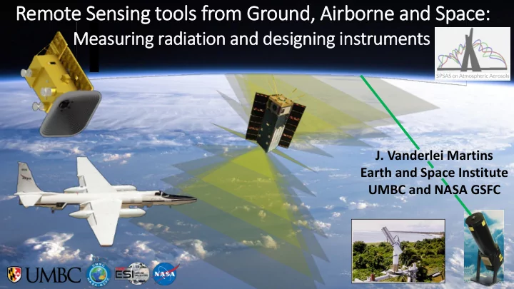
Remote Sensing tools from Ground, Airborne and Space: Measuring - - PowerPoint PPT Presentation

Remote Sensing tools from Ground, Airborne and Space:

Measuring radiation and designing in instruments

• J. Vanderlei Martins

Earth and Space Institute UMBC and NASA GSFC

July 22, 2019 ESI members support and participate in the Sao Paulo Aerosol school at the Institute of Physics of the University of Sao Paulo, Brazil. April 24, 2019 HARP2 passes Critical Design Review at NASA Goddard December, 2018 Several ESI Students and Scientists participate in the AGU Conference in DC

https://esi.umbc.edu/

My current home:

Unique Aircraft In Instrumentation

PI PI-Neph

Platforms: Ground based, Langley B200, NASA P3, NASA DC8 Experiments: DEVOTE, DC3, DISCOVER-AQ CA, STEAR, DISCOVER-AQ CO, STEAR, SEAC4RS, DISCOVER-AQ CO, UMBC Humidification Measurements

NASA ER2 - Oct 2017

OI OI-Neph (NASA P3)

Cloudbow inside a water cloud

HARP Polarimeter Family:

HARP VNIR Telescope

HARP CubeSat – New Technology for Future Missions

5

HARP Prism

SDL Spacecraft UMBC Sensor

HARP Stripe Filter

Funded by NASA-ESTO InVEST Program

Wide FOV Optics Camera and FPGA Electronics

Multi-Angle Observation Multiple Angles Notice that sunglint Is not visible in all angles Sunglint peak No sunglint

• J. Vanderlei Martins – Dept. of Physics, JCET and ESI - UMBC

http://esi.umbc.edu

Thank you!!!

HARP2 on HARP2 on P PACE CE

Passed CDR Review 4/24/2019

HARP2 on PACE Satellite – Launch 2023

The electromagnetic spectrum

Near Infrared (NIR)= 0.7-1.3  m Short wave infrared SWIR = 1.3-2.3 m Mid wave Infrared (MWIR) = 2.3-4 m Thermal IR (TIR) = 4-14 m, Far IR or extreme IR = 14 - 300 m Microwave = 1mm-1m m

Practical but somewhat arbitrary IR classification that I like:

Atmospheric scatterers

size < > ≈ wavelength Wavelength Frequency Air molecules ~0.0004 µm Most aerosol (>0.01 µm) Cloud drops (~ 5-10 µm) Rain drops Ice crystals (hail, etc.)

฀

Coarse aerosol ( sand, dust, sea salt)

Spectral Characteristics of Atmospheric Transmission and Sensing Systems

Solar Spectrum at different levels:

http://lasp.colorado.edu/sorce/instruments/sim/sim_science.htm

Phase Function diagrams for aerosols

q (Scattering Angle)

Incident radiation .021 .063

Size Parameter:

2𝜌 ∙ 𝑠𝑏𝑒𝑗𝑣𝑡 𝑥𝑏𝑤𝑓𝑚𝑓𝑜𝑕𝑢ℎ

Phase Function diagram for Rayleigh scattering

Polarized Components Total Radiation

Observing geometry from Space:

Solar zenith angle Sensor zenith angle Solar view angle Sensor view angle

Basic ic Concepts of Radiation Scattering

• Dr. Luca Lelli – University of Bremen

• Dr. Luca Lelli – University of Bremen

• Dr. Luca Lelli – University of Bremen

Slide Credit: Dr. Luca Lelli – University of Bremen

• Dr. Luca Lelli – University of Bremen

(We also define: bscatt and babs) b

Other important parameters:

• wo (single scattering albedo)
• Probability of scattering over extinction
• Ratio between scattering coefficient and extinction coefficient
• g (asymmetry parameter):
• Defines the fraction of radiation scattered in the forward versus backward

direction

wo = bscatt/bext

Illustration of scattering process

Effect of Single Scattering Albedo Effect of asymmetry parameter

Slide credit: Dr. Luca Lelli – University of Bremen

Slide credit: Dr. Luca Lelli – University of Bremen

Slide credit: Dr. Luca Lelli – University of Bremen

• Dr. Luca Lelli – Un. of Bremen

• Dr. Luca Lelli – Uni. of Bremen

• Dr. Luca Lelli – Univ. of Bremen

• Dr. Luca Lelli – Univ. of Bremen

Rainbow Measurements:

• f Cloud Droplet Size Distribution

F-M. Breon, P. Goloub, 1998.

Unpolarized Cloud top reflectance

Cloudbow Measurements for Accurate Effective Radii and variance

• should provide effective radius retrievals at least one order of magnitude more

accurate than current methods, in addition to unprecedented measurements of the width of the droplet distribution.

Reff = 10m 11m 12m

Cloud top polarized reflectance Effective Radius

0.05 Veff = 0.01 0.2

Cloud top polarized reflectance Distribution Width

My first Measurement of Clo loud Mic icrophysics using the Polarized Clo loudbow

Backup Slides:

Rainbow Camera Prototype Measurement Commercial Flight Beijing New York - August 14 2005

Cloudbow:

Almost invisible in the regular picture but stands out in the polarized image!!!

Rainbow Camera Prototype Measurent Comercial Flight Beijing New York - August 14 2005

Scattering Angle Polarized reflectance

Rainbow Camera Prototype Measurement Commercial Flight Beijing New York - August 14 2005

Measurements using a $200 digital camera and a $10 polarizer sheet

HARP - Unique Aerosols and Clo loud Measurements

(a) (b)

Wide DSD Narrow DSD Narrow DSD

Cloud Droplet Size Retrievals

Back to Aerosols

Aerosol Particles

Saharan Dust Smoke Cluster Smoke Smoldering Phase Smoke Flaming Phase US Urban Pollution

In Interactions between Aerosols and Molecules with R Radiation:

(a) Black Body Curves

5780 K 255 K

N O R M A LI Z A D F L u X

A B S O R P T I O N %

Small Aerosols

Aerosol Extinction Coef. (m-1)

Large Aerosols

Aerosol Extinction Coef. (m-1)

Fine particles from smoke Coarse dust particles

Visible Near-infrared

Aerosol size determination from space

True Color False Color

RGB

HARP – Unique Aerosol and Cloud Measurements

Arizona Fires During ACEPOL 440nm DoLP Prescribed fire in Arizona 2017

Light Scattering Fundamentals and Measurements

Electromagnetic Waves

• Transverse wave with 2 components E and B
• Does not need material medium to travel
• Propagates with the speed of light in vacuum

E B

E B

E B

Dipole (Molecular) Scattering

Polarization

Scattering Plane

Polarization Perpendicular to Scattering Plane

Polarization

Scattering Plane

Q

Polarization Parallel to Scattering Plane

Polarization

Scattering Plane

Q

Phase Function diagram for Rayleigh scattering

Polarized Components Total Radiation

Wincident (qo, fo) Wscattered (q, f) Dw

q

             

in in in in

V U Q I              

sca sca sca sca

V U Q I

f scatterers

Gergely Dolgos, J. Vanderlei Martins 51

Light Input Scattered Light Stokes Parameters to represent the radiation state Intensity Linear Polatization Circular Polarization

Information from Polarization

Droplet 0.1 m Droplet 0.5 m Droplet 1.0 m

Visible light

Color Image Reconstruction

IoE 184 - The Basics of Satellite Oceanography. 3. Remote Sensing of the Sea

• The radiances are measured at different wavebands, called “channels”.
• Different channels provides information on different properties of the Earth’ surface.
• One method of analysis is when the images observed at different wavebands can be

combined to result in a “true color image”.

Image processing RGB Image

Image processing

IoE 184 - The Basics of Satellite Oceanography. 3. Remote Sensing of the Sea

At this MODIS image of the Mississippi River delta you can see clouds, coastline, river, the zones of phytoplankton bloom and pollution in the coastal

• cean, etc.

Image processing

IoE 184 - The Basics of Satellite Oceanography. 3. Remote Sensing of the Sea

True color images are an important source of information about natural disasters like these wildfires in California in autumn 2003.

What is a digital image?

70 53 41 64 84 85 81 88 91 87 79 77 45 38 59 77 84 86 85 85 80 82 69 44 32 45 72 86 82 78 88 79 86 87 65 40 41 75 79 78 93 86 93 106 106 84 56 43 58 75 104 104 100 101 95 91 83 51 39 56 105 110 97 88 84 85 87 77 59 44 96 103 89 79 79 75 77 79 74 72 87 93 97 90 82 76 70 67 61 71 79 81 88 97 93 85 78 74 70 72 81 75 78 85 94 97 92 84 80 72

What your computer sees…

Pixel Digital Number (DN)

8-bit (0 - 255) 9-bit (0 - 511) 10-bit (0 - 1023)

1 2 3 4 1 2 4 8 16 32 64 128

• The sensitivity of remote sensing detectors to differences in

signal strength as it records the radiant flux.

Radiometric Resolution

• These digital numbers will be calibrated to absolute

fluxes [W m-2 m-1] or radiances [W m-2 sr -1 m-1]

Consiglio Nazionale delle Ricerche

ALI 30m 9 bands Hyperion 30m 242 bands TM 30m 6 bands ASTER 15m VNIR, 30m SWIR 9 bands MIVIS 8m 102 bands IKONOS 4m 4 bands

Michael Abrams, Jet Propulsion Laboratory

Examples of imaging capabilities

Spectral Resolution

Only one band covering BGR visible range called panchromatic

Classes of Spectral Imagers

Airborne Visible Infrared Imaging Spectrometer (AVIRIS) Datacube of Sullivan’s Island Obtained

• n October 26, 1998

Color-infrared color composite on top

• f the datacube was

created using three

• f the 224 bands

at 10 nm nominal bandwidth.

1m = 106 m = 1010nm

Image processing

Fine particles from smoke Coarse dust particles

Visible Near-infrared

Aerosol size determination from space

True Color False Color

Generalized Spectral Reflectance Envelopes for Deciduous and Coniferous Trees

Vegetation reflection

Nice indicator for vegetation: Normalized Difference Vegetation Index (NDVI)

฀ NDVI = RNIR − RVIS RNIR + RVIS

Spectral dependence

Typical Spectral Reflectance Curves for Vegetation, Soil, and Water

Vegetation Spectral Properties:

฀ NDVI = RNIR − RVIS RNIR + RVIS

Radiation measurements from the ground

In preparation for our experimental measurement’s day we will focus on SunPhotometers and Sky Radiometers In particular the NASA AERONET system: https://aeronet.gsfc.nasa.gov/

https://youtu.be/i_CJW3JsBI4

Observations Numerical inversion:

• Accounting for noise
• Solving Ill-posed problem
• Setting a priori constraints

Forward model:

• Spectral and angular scattering by particles

with different sizes, compositions and shapes

• Accounting for multiple scattering in atmosphere

aerosol particle sizes, refractive index, single scattering albedo, etc.

Retrieval scheme:

(Dubovik and King, JGR, 2000)

• Direct solar
• Almucantar
• Principal Plane Scan

0.01 0.1 1 10 100 1000 20 40 60 80 100 120 140

Almucantar Fitting Intensity

Scattering Angle (degree) Int(0.44) * 1000 Int(0.67) * 100 Int(0.87) * 10 Int(1.02)

0.1 0.2 0.3 0.4 0.5 0.40 0.60 0.80 1.0 Measurements Fitting Optical thickness Wavelenths (micron)

0.05 0.1 0.15 0.2 0.25 0. 1 10

Retireved size distribution

Radius (microns) m3/m2)

1.35 1.40 1.45 1.50 1.55 1.60

Wavelength ( m)

0.44 0.67 0.87 1.02

Real Part

0.00 0.01 0.10

Wavelength ( m)

0.44 0.67 0.87 1.02

Imarinary Part

Imaginary Part

Fitting as a retrieval strategy

Refractive Indices AOD Size Distribution

The averaged optical properties of various aerosol types

(Dubovik et al., 2002, JAS)

Utilizing polarization

Cape Verde aerosol

dV/dln(ri) n(l) w0(l)

Principal Plane: t(l), I(l,Q) l = 0.44, 0.5, 0.67, 0.87,1.02, 1.64, m

0.02 0.04 0.06 0.08 0.1 0.12 0.14 0.1 1 10

almucantar principle plane 0.87 m(with polarization) principle plane (4 channels + polarization) dV/dlnR ( m

3/m 2)

Particle Radius (micron)

28:09: 2003,18:07:54,Principal_Plane,Capo_Verde,47

1.3 1.35 1.4 1.45 1.5 1.55 1.6 1.65 0.4 0.5 0.6 0.7 0.8 0.9 1

almucantar principle plane 0.87 m(with polarization) principle plane (4 channels + polarization) Real Part of Reffactive Index Wavelengths ( m)

28:09: 2003,18:07:54,Principal_Plane,Capo_Verde,47

0.6 0.7 0.8 0.9 1 0.4 0.5 0.6 0.7 0.8 0.9 1 1.1

almucantar principal plane (radiances) principal plane (polarization, 0.87 m) principal plane (4 channels + polar) Single Scattering Albedo Wavelengths ( m)

28:09: 2003,18:07:54,Principal_Plane,Capo_Verde,47

Polarization : t(l), I(l,Q),P(l,Q) l = 0.87m

Fitting polarization

Radiance Linear Polarizartion

Cape Verde aerosol

0.01 0.1 1 10 30 60 90 120 150

Measurements Fitting

Radiance in Principle Plane Scattering Anlge (degrees)

0.1 0.2 0.3 0.4 0.5 0.6 50 75 100 125 150

Measurements Fitting

Linear Polarization (-F

12/F 11)

Scattering Anlge (degrees)

Fine and Coarse modes separations

Radiance

Beijing aerosol

0.1 1 10 100 45 90 135 180

total fine mode coarse mode

Phase Function Particle Radius (micron)

02:05: 2003,09:27:51,PolarPP,Beijing,14

0.3 0.6 0.9 45 90 135 180

total fine mode coarse mode

Linear Polarization (-F

12/F 11)

Particle Radius (micron)

02:05: 2003,09:27:51,PolarPP,Beijing,14

0.02 0.04 0.06 0.08 0.1 0.12 0.14 0.1 1 10

dV/dlnR ( m

3/m 2)

Particle Radius (micron) Coarse Fine Coarse

02:05: 2003,09:27:51,PolarPP,Beijing,14

Beijing Aerosol

Flexible separation between fine and coarse modes (curently: ~0.6 m)

0.45m

Retrieval using combinations of up-looking Ground-based and down-looking satellite

• bservations

Retrieved: Aerosol Properties:

• size distribution
• real ref. ind.
• imag. ref. ind

(AERONET sky channels)

Surface Parameters:

• BRDF (MISR channels)
• Albedo (MODIS IR channels)

Phase Function diagram for Rayleigh scattering

Polarized Components Total Radiation

Observing geometry from Space:

Solar zenith angle Sensor zenith angle Solar view angle Sensor view angle

Field Measurement’s Day

• Prof. J. Vanderlei Martins

Earth and Space Institute – UMBC University of Maryland Baltimore County

Our Experimental Measurement’s day:

• Field trip to the MAC (Contemporaneous Art

Museum)

• Measurements from the roof top of the

building observing solar and sky radiances with a simple manual photometer from your smart phone.

• The intent is to illustrate how to make

measurements and convert it to scientific variables but it is not to actually perform a fully calibrated scientific measurement

• First you will characterize and understand

better the sensors in your Smart Phone:

• Photometer
• Camera
• Inclinometers, accelerometers, compass, GPS, etc.
• Second you will perform actual atmospheric

measurements and compare results with AERONET

Ibirapuera Park Across the Street from MAC

What to bring:

• We plan to use personal Smart phones

for the measurement

• Students will be divided in teams of 3

people

• Important to have at least one

smartphone per team

• Not required but very useful to have a

laptop computer for data analysis (plotting, etc.).

• Sunscreen, hat, long sleeves for wind

and sun blocking

• Water bottle or mug.
• Lunch boxes will be provided by the

School.

Important notes:

• The museum is a safe/secure place but, keep in mind that you are

bringing smartphones, laptops and other belongings at your own risk.

• You can visit the whole museum but our experimental activities will

happen only the 1st and 8th floors.

• Across the street from the museum there is the beautiful Ibirapuera

Park that you should consider visiting. While in the Park be always careful with your belongings (computer, cameras, phones, etc.).

Important: You are not allowed to bring backpacks to any other floors!!! In fact, it is better to keep your backpacks in the 1st floor rooms dedicated to our group.

Apps to download to your computer:

• There are three Apps that we plan to

use in this experiment:

• Physics toolbox suite
• GPS Status
• Photometer PRO –

Lux Light Meter & Tools

Note: Aple Iphone’s will have a different photometer App but it should work similarly

If your phone is limited in memory space, start with the Photometer Pro – Lux Light Meter. You may be able to use this App only for all measurements.

Division in groups

• Students will be divided in teams of 3 people
• There must be at least one smartphone per team.
• It would be useful if each team had at least one laptop computer for data

analysis.

• The student teams will be split into 4 groups lead by a professor and

monitors.

• The Professors will coordinate the groups to perform experimental

activities in the laboratories and on the roof of the museum.

• Each group will have an assigned 2 hours window to perform the

laboratory characterization of their phone.

Computer and Data analysis

• A laptop computer is not required for participation in the course but

it is highly recommended.

• We will have data analysis and measurement activities for which the

laptop computer will be highly beneficial. The work will be done in groups of 3 students so, it is highly advisable to have at least one computer in each group.

Software requirements

• Any data analysis software (including excel) can be used to the

general data analysis but we will be basin all our measurements and data analysis on Python.

• I highly recommend everybody to install and get some familiarity with
• Python. In particular, I recommend Python 2.7 in the Anaconda

distribution.

Poster Session

• Student teams will prepare a poster with results from their

experiment to present to the whole group of students. We will have a poster session in the last Thursday of the event.

Ext xtra sli lides

‘s Image Gallery

for ACEPOL

Oct 25th Nov 1st Nov 7th Oct 27th Oct 26th Oct 23rd Oct 19th Nov 3rd Nov 9th Nov 9th

(Level 1 data under processing)

UMBC AirHARP and AirSPEX from ER2

NASA ACEPOL – Nov 2018

Evaluating this relationship on the solar principal plane gives the effective radius (reff) and variance (veff) of a cloud scene from the recovered Mie P12. HARP cloud retrievals can be done for any pixel in the FOV, even for heterogeneous clouds, like this case (left) from LMOS on June 19, 2017. Polarized radiance is converted to reflectance (Rp) and parametrically matched to Mie phase functions: 𝑆𝑄 = 𝜌 𝑅2 + 𝑉2 𝐺

0 cos 𝜘𝑨

= 𝛽 𝑄

12 𝜘 + 𝛾𝑑𝑝𝑡2𝜄 + 𝛿

Level 2 retrieval algorithms and adaptation of HARP data to GRASP for aerosol retrieval are underway.

AirHARP 670nm 10x10 super-pixel retrieval (80m total grd. res.) Retrieved Parameters Reff = 6.0um Veff = 0.03

LMOS

AirHARP RP • Best Parametric Fit - - -

Intensity Polarization

HARP Pioneering Hyper-Angular Capability from Space will Provide Full Cloudbow Retrievals from Small Area (~4x4km)

Intensity Polarization 98

HARP Pioneering Hyper-Angular Capability will Provide Full Cloudbow Retrievals from Small Area (< 4x4km from space)

HARP CubeSat Polarimeter

Intensity Polarization

D A

D and A produce cloud droplet effective radius and variance

Water Droplet Distribution

Reff = 20m Veff = 0.01 Reff = 20m Veff = 0.09 Effective Radius (m) These two cases are undistinguishable from Intensity measurements only (MODIS/VIIRS)

HyperAngular High Resolution Cloudbow

DoLP Intensity 1 km

Scattering Angle Cloud Hole Cloudy pieces Stokes parameters

Evaluation of Cloud 3D Properties

LES and 3D RT simulations by Chamara Rajapakshe and Zhibo Zhang AirHARP Data Set by Vanderlei Martins, Brent McBride and H. Barbosa