Recapitulation What do we want? v = disturbance y u System e = - - PowerPoint PPT Presentation

Recapitulation

What do we want?

System

• u

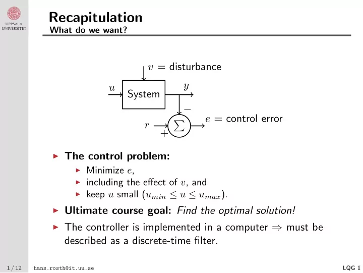
y − r + e = control error v = disturbance

◮ The control problem:

◮ Minimize e, ◮ including the effect of v, and ◮ keep u small (umin ≤ u ≤ umax).

◮ Ultimate course goal: Find the optimal solution! ◮ The controller is implemented in a computer ⇒ must be

described as a discrete-time filter.

1 / 12 hans.rosth@it.uu.se LQG 1

Recapitulation, cont’d

What have we achieved? — summary of what we have looked at so far

◮ Discrete-time systems:

◮ Difference equations, ◮ shift operator q, ◮ stability region = inside of the unit circle.

◮ Sampling of systems = zero-order hold sampling (ZOH):

◮ Exact for t = kh, ◮ sampling period = h, ◮ Nyquist frequency ωn = ωs/2 = π/h, ◮ frequency response of G(z) for z = eiωh.

◮ MIMO systems: Straightforward to use state space forms. ◮ Disturbance models:

◮ Spectral density: Φ(ω) = F[r(τ)], ◮ white noise v ⇔ Φv(ω) = Rv = const., ◮ linear filtering: y = Gu ⇒ Φy = |G|2Φu, ◮ spectral factorization: Φ = |G|2R, ◮ Lyapunov equation ⇒ Πx = ExxT .

◮ Kalman filters: Optimal observer, Riccati equations (CARE,

DARE).

2 / 12 hans.rosth@it.uu.se LQG 1

Optimal control design: LQG

Starting point in the continuous-time case

◮ Use the “standard” state space representation

     ˙ x = Ax + Bu + Nv1, z = Mx, y = Cx + v2, η = v1 v2

• , Φη(ω) =

R1 R12 RT

12

R2

• ◮ Minimize the criterion

V = ||z||2

Q1 + ||u||2 Q2 ◮ The weighting matrices,

Q1 = QT

1 ≥ 0

and Q2 = QT

2 > 0,

are design parameters.

3 / 12 hans.rosth@it.uu.se LQG 1

Optimal control

Interpretations of the criterion

◮ || · ||2 Q is a squared weighted signal norm, a measure of size of

the signal (cf. mean power, energy etc.).

◮ Stochastic setting (v1, v2 = 0), version 1:

V = E

• zT Q1z + uT Q2u
• ◮ ... version 2 — “empirical” interpretation:

V = lim

T→∞

1 T T

• zT Q1z + uT Q2u
• dt

◮ Deterministic setting (v1 = 0 and v2 = 0):

V = ∞

• zT Q1z + uT Q2u
• dt

4 / 12 hans.rosth@it.uu.se LQG 1

Control strategy

State feedback with observer

The optimal controller is conveniently represented as state feedback from estimated states.

◮ Control law: u(t) = −Lˆ

x(t) + ˜ r(t)

◮ Observer: ˙

ˆ x(t) = Aˆ x(t) + Bu(t) + K(y(t) − Cˆ x(t))

◮ The control law can also be written as

     U(s) = Fr(s) ˜ R(s) − Fy(s)Y (s), Fy(s) = L(sI − A + BL + KC)−1K, Fr(s) = I − L(sI − A + BL + KC)−1B

◮ The poles of the closed loop system are the roots of

0 = det(sI − A + BL) · det(sI − A + KC), i.e. poles from state feedback + the observer poles.

5 / 12 hans.rosth@it.uu.se LQG 1

Observer based state feedback control

Example: A DC-motor

1 s(s+1)

• u

v1 z v2 y                ˙ x =

• −1

1

• x +
• 1
• u +
• 1
• v1

z =

• 1
• x

y =

• 1
• x + v2

state feedback: u = −Lˆ x + Lrr L =

• l1

l2

• ˆ

x from observer Closed loop system: Z(s) = Gc(s)LrR(s) + G(s)S(s)V1(s) − T(s)V2(s) Gc(s) = M(sI − A + BL)−1B = b(s) p(s) = 1 s2 + (1 + l1)s + l2

6 / 12 hans.rosth@it.uu.se LQG 1

LQG: The optimal controller

Theorem 9.1

◮ The optimal control law is u(t) = −Lˆ

x(t),

◮ ˆ

x(t) is obtained from the corresponding Kalman filter.

◮ The optimal state feedback gain is

L = Q−1

2 BT S, ◮ the matrix S = ST ≥ 0 is the solution to the continuous-time

algebraic Riccati equation (CARE) 0 = AT S + SA + MT Q1M − SBQ−1

2 BT S ◮ Some technical conditions: (A, B) stabilizable, (A, C) and

(A, MT Q1M) detectable...

◮ N.B. There are two different CAREs involved, the one above

and the one for the Kalman filter!

7 / 12 hans.rosth@it.uu.se LQG 1

LQG & the Kalman filter

Comparison of Riccati equations — duality

A CARE again!

◮ The Kalman filter (with R12 = 0): K = PCT R−1 2

0 = AP + PAT + NR1NT − PCT R−1

2 CP ◮ The LQG state feedback gain: L = Q−1 2 BT S

0 = AT S + SA + MT Q1M − SBQ−1

2 BT S

A comparison: KF: A N C R1 R2 P K

• LQ:

AT MT BT Q1 Q2 S LT

8 / 12 hans.rosth@it.uu.se LQG 1

LQ/LQG: Properties

◮ A − BL is always stable ◮ The control law u(t) = −Lx(t) (pure state feedback) is

• ptimal, also for the deterministic case (v1 = 0 and v2 = 0)

⇔ LQ = linear quadratic control.

◮ If v1 and v2 have Gaussian distributions the controller is the

• ptimal controller (Cor. 9.1) ⇔ LQG = linear quadratic

Gaussian control.

◮ Theorem 9.1 = the separation theorem:

The optimal observer = the Kalman filter, combined with the

• ptimal state feedback (LQ) give the optimal controller! (This

is far from obvious...)

◮ The LQ/LQG controller looks exactly the same for SISO and

MIMO systems.

9 / 12 hans.rosth@it.uu.se LQG 1

LQ example

The DC-motor

Deterministic case (LQ): u = −Lx + Lrr A = −1 1

• ,

B = 1

• ,

M =

• 1
• ,

S = s1 s12 s12 s2

• The CARE 0 = AT S + SA + MT Q1M − SBQ−1

2 BT S, spelled out:

• =

−s1 + s12 −s12 + s2

• +

−s1 + s12 −s12 + s2

• +

Q1

• − 1

Q2 s2

1

s1s12 s1s12 s2

12

• The solution is

S = Q2 √1 + 2ρ − 1 ρ ρ ρ√1 + 2ρ

• with

ρ =

• Q1

Q2 and L = Q−1

2 BT S = 1

Q2

• s1

s12

• =

√1 + 2ρ − 1 ρ

• 10 / 12

hans.rosth@it.uu.se LQG 1

The servo problem

How can the reference signal r(t) be included?

◮ General solution: Characterize r(t) by its spectrum and model

it in the same way as a disturbance, i.e. incorporate it in the model.

◮ Special case, Theorem 9.2: If r(t) is piecewise constant,

then the criterion V = ||z − r||2

Q1 + ||u − u∗(r)||2 Q2

is minimized with the control law u(t) = −Lˆ x(t) + Lrr(t), where L and ˆ x(t) are given as in Theorem 9.1, and Lr is chosen so that I = M(sI − A + BL)−1BLr

• s=0 = Gc(0)Lr.

(Then u∗(r) = Lrr.)

11 / 12 hans.rosth@it.uu.se LQG 1

Example: LQ control of a DC-motor

The effect of Q1 and Q2

◮ The DC-motor: Y (s) = 1 s(s+1)U(s)

Design parameters: Q1 = 1, Q2 = 1 / 0.1 / 0.01 LQ control ⇒ pure state feedback: u(t) = −Lx(t) + Lrr(t)

◮ Simulations: Step responses for the closed loop systems.

◮ The outputs, y:

Q2 = 1 Q2 = 0.1 Q2 = 0.01

◮ The inputs, u:

Q2 = 1 Q2 = 0.1 Q2 = 0.01

12 / 12 hans.rosth@it.uu.se LQG 1