Recapitulation: Expected Measurements innovation statistics, - - PowerPoint PPT Presentation

SLIDE 1

Recapitulation: Expected Measurements

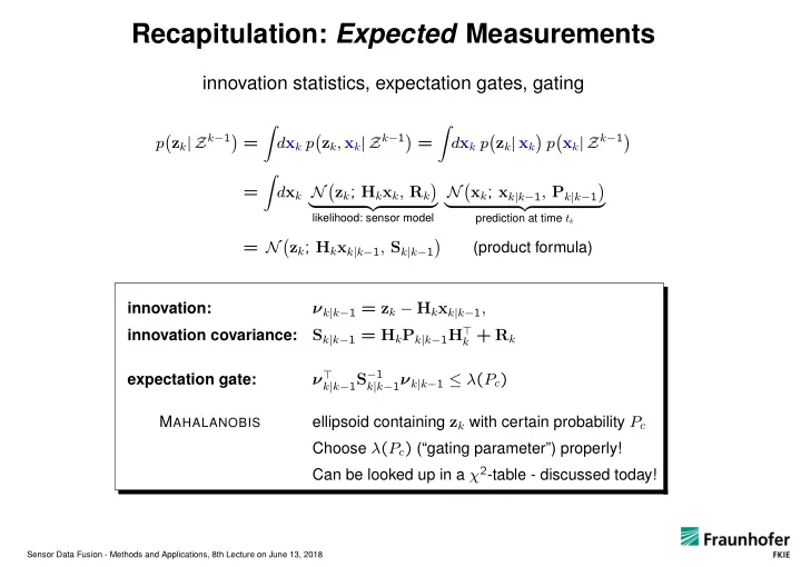
innovation statistics, expectation gates, gating

pzk| Zk1 =

Z

dxk pzk, xk| Zk1 =

Z

dxk pzk| xk

• pxk| Zk1

=

Z

dxk N

• zk; Hkxk, Rk
• |

{z }

likelihood: sensor model

N

• xk; xk|k1, Pk|k1
• |

{z }

prediction at time tk

= N

• zk; Hkxk|k1, Sk|k1
• (product formula)

innovation:

νk|k1 = zk Hkxk|k1,

innovation covariance:

Sk|k1 = HkPk|k1H>

k + Rk

expectation gate:

ν>

k|k1S1 k|k1νk|k1  (Pc)

MAHALANOBIS ellipsoid containing zk with certain probability Pc Choose (Pc) (“gating parameter”) properly! Can be looked up in a 2-table - discussed today!

Sensor Data Fusion - Methods and Applications, 8th Lecture on June 13, 2018

SLIDE 2

Sensor data of uncertain origin

• prediction: xk|k1, Pk|k1 (dynamics)
• innovation: νk = zk Hxk|k1 , white
• Mahalanobis norm: ||νk||2 = ν>

k S1 k νk

• expected plot: zk ⇠ N(Hxk|k1, Sk)
• νk ⇠ N(0, Sk), Sk = HPk|k1H>+R
• gating: ||νk|| < , Pc() correlation prob.

missing/false plots, measurement errors, scan rate, agile targets: large gates

Sensor Data Fusion - Methods and Applications, 8th Lecture on June 13, 2018

SLIDE 3

Sensor Data Fusion - Methods and Applications, 8th Lecture on June 13, 2018

SLIDE 4

Sensor Data Fusion - Methods and Applications, 8th Lecture on June 13, 2018

SLIDE 5

Sensor Data Fusion - Methods and Applications, 8th Lecture on June 13, 2018

SLIDE 6

Sensor Data Fusion - Methods and Applications, 8th Lecture on June 13, 2018

SLIDE 7

Sensor Data Fusion - Methods and Applications, 8th Lecture on June 13, 2018

SLIDE 8

Sensor Data Fusion - Methods and Applications, 8th Lecture on June 13, 2018

SLIDE 9

Sensor Data Fusion - Methods and Applications, 8th Lecture on June 13, 2018

SLIDE 10

Sensor Data Fusion - Methods and Applications, 8th Lecture on June 13, 2018

SLIDE 11

Sensor Data Fusion - Methods and Applications, 8th Lecture on June 13, 2018

SLIDE 12

Sensor Data Fusion - Methods and Applications, 8th Lecture on June 13, 2018

SLIDE 13

Sensor Data Fusion - Methods and Applications, 8th Lecture on June 13, 2018

SLIDE 14

Sensor Data Fusion - Methods and Applications, 8th Lecture on June 13, 2018

SLIDE 15

Sensor Data Fusion - Methods and Applications, 8th Lecture on June 13, 2018

SLIDE 16

Sensor Data Fusion - Methods and Applications, 8th Lecture on June 13, 2018

SLIDE 17

Sensor Data Fusion - Methods and Applications, 8th Lecture on June 13, 2018

SLIDE 18

Sensor Data Fusion - Methods and Applications, 8th Lecture on June 13, 2018

SLIDE 19

Sensor Data Fusion - Methods and Applications, 8th Lecture on June 13, 2018

SLIDE 20

DEMONSTRATION

Sensor Data Fusion - Methods and Applications, 8th Lecture on June 13, 2018

SLIDE 21

Likelihood Functions

The likelihood function answers the question: What does the sensor tell about the state x of the object? (input: sensor data, sensor model)

• ideal conditions, one object: PD = 1, ⇢F = 0

at each time one measurement:

p(zk|xk) = N(zk; Hxk, R)

• real conditions, one object: PD < 1, ⇢F > 0

at each time nk measurements Zk = {z1

k, . . . , znk k }! p(Zk, nk|xk) / (1 PD)⇢F + PD

nk

X

j=1

Nzj

k; Hxk, R

21 Introduction to Sensor Daten Fusion: Methods and Applications — 8th Lecture on June 13, 2018

SLIDE 22

PDAF Filter: formally analog to Kalman Filter

Filtering (scan k1): p(xk1|Zk1) ⇡= N(xk1; xk1|k1, Pk1|k1) (! initiation) prediction (scan k): p(xk|Zk1) ⇡ N(xk; xk|k1, Pk|k1) (like Kalman) Filtering (scan k): p(xk|Zk) ⇡

mk

X

j=0

pj

k N(xk; xj k|k, Pj k|k) ⇡ N(xk; xk|k, Pk|k)

νk

=

Pmk

j=0 pj k νj k ,

νj

k

= zj

k Hxk|k1

combined innovation

Wk

= Pk|k1H>S1

k ,

Sk

= HPk|k1H> + Rk Kalman gain matrix pj

k

= pi⇤

k / P j pj⇤ k ,

pj⇤

k

=

(

(1 PD) ⇢F

PD

p

|2⇡Sj| e 1

2ν> j S1 j νj

weighting factors

xk = xk|k1 + Wk νk

(Filtering Update: Kalman)

Pk = Pk|k1 (1p0

k) WkSW> k

(Kalman part) + Wk

n Pmk

j=0 pj k νj kνj> k

νkνk>o

W>

k

(Spread of Innovations)

22 Introduction to Sensor Daten Fusion: Methods and Applications — 8th Lecture on June 13, 2018

SLIDE 23

Refined Sensor Modeling: Resolution Phenomena

• band/beam width, coherence:

e.g. for RADAR: ↵r = 200 m, ↵' = 2, ↵˙

r = 2 m/s

• irresolved measurement:

Hg xk = 1

2 H(x1 k + x2 k)

“center of gravity”

• resolution (qualitatively):

· depending on target-sensor geometry, rel. orientation · resolution capability in r, ', ˙ r mutually independent · very low resolution for: ∆r<↵r, ∆'<↵', ∆˙ r<↵˙

r

· no resolution phenomena: ∆r↵r, ∆'↵', ∆˙ r↵˙

r

· small transient region between these domains

Sensor Data Fusion - Methods and Applications, 8th Lecture on June 13, 2018

SLIDE 24

Refined Sensor Modeling: Resolution Phenomena

• band/beam width, coherence:

e.g. for RADAR: ↵r = 200 m, ↵' = 2, ↵˙

r = 2 m/s

• irresolved measurement:

Hg xk = 1

2 H(x1 k + x2 k)

“center of gravity”

• resolution (qualitatively):

· depending on target-sensor geometry, rel. orientation · resolution capability in r, ', ˙ r mutually independent · very low resolution for: ∆r<↵r, ∆'<↵', ∆˙ r<↵˙

r

· no resolution phenomena: ∆r↵r, ∆'↵', ∆˙ r↵˙

r

· small transient region between these domains

• Echelon formation:

Sensor Data Fusion - Methods and Applications, 8th Lecture on June 13, 2018

SLIDE 25

Refined Sensor Modeling: Resolution Phenomena

• band/beam width, coherence:

e.g. for RADAR: ↵r = 200 m, ↵' = 2, ↵˙

r = 2 m/s

• irresolved measurement:

Hg xk = 1

2 H(x1 k + x2 k)

“center of gravity”

• resolution (qualitatively):

· depending on target-sensor geometry, rel. orientation · resolution capability in r, ', ˙ r mutually independent · very low resolution for: ∆r<↵r, ∆'<↵', ∆˙ r<↵˙

r

· no resolution phenomena: ∆r↵r, ∆'↵', ∆˙ r↵˙

r

· small transient region between these domains

• a simple resolution model:

Pr(∆r, ∆', ∆˙ r) = 1Pu(∆r, ∆', ∆˙ r) Pu = e log 2( ∆r

↵r )2 e log 2( ∆' ↵' )2 e log 2( ∆˙ r ↵˙ r )2

= |2⇡Ru|

1 2 N

• O; H(x1

k x2 k), Ru

• Sensor Data Fusion - Methods and Applications, 8th Lecture on June 13, 2018

SLIDE 26

Interpretation hypotheses:

`(Zk, nk|xk) = P

Ek `(Zk, nk, Ek|xk)

• Eii

k : Objects irresolved, detected as a group, zi k 2 Zk being the plot:

`(Zk, nk, Eii

k |xk) = const. ⇥ Pu(xk) N(zi k; Hg kxk, Rg k)

= const.0 ⇥ N

✓✓ zi

k

• ◆

;

✓ Hg

k

Hu ◆

xk,

✓ Rg

k O

O Ru ◆◆

Assuming Eii

k , we process a (real) measurement zi k of the center

1 2H(x1 k + x2 k) and a (fictitious) measurement “zero” of the distance

H(x1

k x2 k) between the targets. Ru defines the resolution capability.

Sensor Data Fusion - Methods and Applications, 8th Lecture on June 13, 2018

SLIDE 27

Interpretation hypotheses:

`(Zk, nk|xk) = P

Ek `(Zk, nk, Ek|xk)

• Eii

k : Objects irresolved, detected as a group; zi k 2 Zk being the plot `(Zk, nk, Eii

k |xk) = const. ⇥ N

⇣⇣

zi

k

• ⌘

;

⇣

Hg

k

Hu

⌘ xk, ⇣

Rg

k O

O Ru

⌘⌘

• E00

k : Objects neither resolved, nor detected; all plots are false

`(Zk, nk, E00

k |xk) = Pu(xk) (1P u D) pF (nk) |FoV|nk

= const. ⇥ N

⇣

O; H(x1

k x2 k), Ru

⌘

Assuming E00

k , a fictitious zero-distance measurement is processed.

Sensor Data Fusion - Methods and Applications, 8th Lecture on June 13, 2018

SLIDE 28

Interpretation hypotheses:

`(Zk, nk|xk) = P

Ek `(Zk, nk, Ek|xk)

• Eii

k : Objects irresolved, detected as a group, zi k 2 Zk being the plot `(Zk, nk, Eii

k |xk) = const. ⇥ N

⇣⇣

zi

k

• ⌘

;

⇣

Hg

k

Hu

⌘ xk, ⇣

Rg

k O

O Ru

⌘⌘

• E00

k : Objects neither resolved, nor detected; all plots are false `(Zk, nk, E00

k |xk) = const. ⇥ N

• O; H(x1

k x2 k), Ru

• Eij

k : Objects resolved and individually detected, zi k, zj k being the plots `(Zk, nk|Eij

k , xk) = const. ⇥

⇥

1Pu(xk)

⇤

N

⇣⇣

zi

k

zj

k

⌘

;

Hk

Hk

• xk,

Rk O

O Rk

⌘

Mixtures with negative coefficients occur! Interpretation: Resolved targets keep a minimum distance, otherwise they were irresolvable.

Sensor Data Fusion - Methods and Applications, 8th Lecture on June 13, 2018

SLIDE 29

radar raw data no resolution model with resolution model

Sensor Data Fusion - Methods and Applications, 8th Lecture on June 13, 2018

SLIDE 30

Unresolved measurement zu

k of a group of n closely spaced targets: group centroid

p(zu

k|x1:n k

) = N

⇣

zu

k; Hgx1:n k

, Rg

⌘

,

x1:n

k

= (x1

k, . . . xn k)

Rg: measurement error of unresolved measurements; measurement matrix: Hg = Hk ⌦ (1, . . . 1).

Sensor Data Fusion - Methods and Applications, 8th Lecture on June 13, 2018

SLIDE 31

Unresolved measurement zu

k of a group of n closely spaced targets: group centroid

p(zu

k|x1:n k

) = N

⇣

zu

k; Hgx1:n k

, Rg

⌘

,

x1:n

k

= (x1

k, . . . xn k)

Rg: measurement error of unresolved measurements; measurement matrix: Hg = Hk ⌦ (1, . . . 1).

Probability of being unresolved Pu(x1:n

k

): pseudo measurements “zero” of the distances, sensor resolution, e.g. ↵r, ↵xr, as pseudo measurement error covariance: Pu(x1:n

k

) = |2⇡Ru|

1 2 N

⇣

0; Hdx1:n

k

, Au

⌘

. Pseudo measurement matrix Hd (mutual distances):

Hd = Hk ⌦

B B B @

1 1 . . . ... ... . . . ... 1 1 1 . . . 1

1 C C C A .

Sensor Data Fusion - Methods and Applications, 8th Lecture on June 13, 2018

SLIDE 32

The notion of identical targets: indistinguishability

Often sensor measurements do not reveal the identity of a target! In general, likelihood functions can be written as sums of partial sums over classes Hµ

k

• f data interpretation hypotheses that differ only in a permutation of the target labels:

`(x1:n

k

; Zk) =

X

µ

`µ(x1:n

k

; Zk) with: `µ(x1:n

k

; Zk) /

X

hk2Hµ

k

p(hk) p(Zk|x1:n

k

, hk).

Sensor Data Fusion - Methods and Applications, 8th Lecture on June 13, 2018

SLIDE 33

The notion of identical targets: indistinguishability

Often sensor measurements do not reveal the identity of a target! In general, likelihood functions can be written as sums of partial sums over classes Hµ

k

• f data interpretation hypotheses that differ only in a permutation of the target labels:

`(x1:n

k

; Zk) =

X

µ

`µ(x1:n

k

; Zk) with: `µ(x1:n

k

; Zk) /

X

hk2Hµ

k

p(hk) p(Zk|x1:n

k

, hk). Symmetry under permutations n of the target labels: 8 2 Sn : `µ(x1:n

k

; Zk) = `µ(x(1:n)

k

; Zk) p(x1:n

l

|Zk:1) = p(x(1:n)

l

|Zk:1)

What about anti-symmetry?

• W. Koch. On Anti-symmetry in Multiple Target Tracking, FUSION 2018, Cambridge, July 2018

Sensor Data Fusion - Methods and Applications, 8th Lecture on June 13, 2018

SLIDE 34

The notion of identical targets: indistinguishability

Often sensor measurements do not reveal the identity of a target! In general, likelihood functions can be written as sums of partial sums over classes Hµ

k

• f data interpretation hypotheses that differ only in a permutation of the target labels:

`(x1:n

k

; Zk) =

X

µ

`µ(x1:n

k

; Zk) with: `µ(x1:n

k

; Zk) /

X

hk2Hµ

k

p(hk) p(Zk|x1:n

k

, hk). Symmetry under permutations n of the target labels: 8 2 Sn : `µ(x1:n

k

; Zk) = `µ(x(1:n)

k

; Zk) p(x1:n

l

|Zk:1) = p(x(1:n)

l

|Zk:1)

What about anti-symmetry?

• W. Koch. On Anti-symmetry in Multiple Target Tracking, FUSION 2018, Cambridge, July 2018

Sensor Data Fusion - Methods and Applications, 8th Lecture on June 13, 2018

SLIDE 35

Two targets in clutter: five classes Hm

k , m = 1, . . . 5, of data interpretation hypotheses:

`(x1:n

k

; Zk) /

5

X

i=1

`i(x1:2

k

; Zk), Zk = {zj

k}mk j=1

H1

k — Both targets resolvable, but not detected; all mk measurements are false

(one interpretation hypothesis): `1(x1:2

k

; Zk) = ⇢2

F(1 PD)2⇣

1 Pu(x1:2

k

)

⌘

.

Sensor Data Fusion - Methods and Applications, 8th Lecture on June 13, 2018

SLIDE 36

Two targets in clutter: five classes Hm

k , m = 1, . . . 5, of data interpretation hypotheses:

`(x1:n

k

; Zk) /

5

X

i=1

`i(x1:2

k

; Zk), Zk = {zj

k}mk j=1

H1

k — Both targets resolvable, but not detected; all mk measurements are false

(one interpretation hypothesis): `1(x1:2

k

; Zk) = ⇢2

F(1 PD)2⇣

1 Pu(x1:2

k

)

⌘

. H2

k — Both targets neither resolvable nor detected as a group, all measurements

are false (one interpretation hypothesis): `2(x1:2

k

; Zk) = ⇢F(1 P u

D)Pu(x1:2 k

).

Sensor Data Fusion - Methods and Applications, 8th Lecture on June 13, 2018

SLIDE 37

Two targets in clutter: five classes Hm

k , m = 1, . . . 5, of data interpretation hypotheses:

`(x1:n

k

; Zk) /

5

X

i=1

`i(x1:2

k

; Zk), Zk = {zj

k}mk j=1

H1

k — Both targets resolvable, but not detected; all mk measurements are false

(one interpretation hypothesis): `1(x1:2

k

; Zk) = ⇢2

F(1 PD)2⇣

1 Pu(x1:2

k

)

⌘

. H2

k — Both targets neither resolvable nor detected as a group, all measurements

are false (one interpretation hypothesis): `2(x1:2

k

; Zk) = ⇢F(1 P u

D)Pu(x1:2 k

). H3

k — Both targets not resolvable but detected as a group with probability P u D, zj k 2 Zk

a the centroid measurement; all remaining returns false (mk data interpretations): `3(x1:2

k

; Zk) = ⇢FP u

DPu(x1:2 k

)

mk

X

j=1

N

⇣

zj

k; Hgx1:2 k

, Rg

⌘

(1) (2)

Sensor Data Fusion - Methods and Applications, 8th Lecture on June 13, 2018

SLIDE 38

H4

k — Both objects were resolvable but only one object was detected, zj k is the

measurement, mk 1 measurements are false (2mk interpretations) with: 4

⇣

zj

k; Hkx1:2 k

, Rj

k

⌘

= N

⇣

zj

k; Hkx1 k, Rj k

⌘

+ N

⇣

zj

k; Hkx2 k, Rj k

⌘

, `4(x1:2

k

; Zk) = ⇢FPD(1 PD) ⇥

⇣

1 Pu(x1:2

k

)

⌘

mk

X

j=1

4

⇣

zj

k; Hkx1:2 k

, Rj

k

⌘

.

Sensor Data Fusion - Methods and Applications, 8th Lecture on June 13, 2018

SLIDE 39

H4

k — Both objects were resolvable but only one object was detected, zj k is the

measurement, mk 1 measurements are false (2mk interpretations) with: 4

⇣

zj

k; Hkx1:2 k

, Rj

k

⌘

= N

⇣

zj

k; Hkx1 k, Rj k

⌘

+ N

⇣

zj

k; Hkx2 k, Rj k

⌘

, `4(x1:2

k

; Zk) = ⇢FPD(1 PD) ⇥

⇣

1 Pu(x1:2

k

)

⌘

mk

X

j=1

4

⇣

zj

k; Hkx1:2 k

, Rj

k

⌘

. H5

k — Both objects were resolvable and detected, zi k, zj k are the measurements,

mk 2 measurements are false (mk(mk 1) interpretations) with: 5

⇣

x1:2

k

; zij

k , Rij k

⌘

= S N

⇣

zij

k ; Hkx1:2 k

, Rij

k

⌘

, `5(x1:2

k

; Zk) = P 2

D

⇣

1 Pu(xk)

⌘

⇥

mk1

X

i=1 mki

X

j=1

5

⇣

x1:2

k

; zij

k , Rij k

⌘

, symmetrizing operator: Sf

⇣

x1:n

⌘

=

X

2Sn

f

⇣

x(1:n)

⌘

,

Sensor Data Fusion - Methods and Applications, 8th Lecture on June 13, 2018