5.3 EXPECTED VALUE AND VARIANCE def: The expected value of a random - - PDF document

Section 5.3 Expected Value and Variance

5.3.1

5.3 EXPECTED VALUE AND VARIANCE

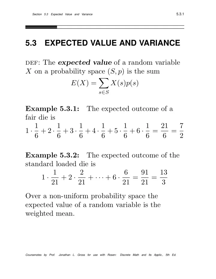
def: The expected value of a random variable X on a probability space (S, p) is the sum E(X) =

• s∈S

X(s)p(s) Example 5.3.1: The expected outcome of a fair die is 1 · 1 6 + 2 · 1 6 + 3 · 1 6 + 4 · 1 6 + 5 · 1 6 + 6 · 1 6 = 21 6 = 7 2 Example 5.3.2: The expected outcome of the standard loaded die is 1 · 1 21 + 2 · 2 21 + · · · + 6 · 6 21 = 91 21 = 13 3 Over a non-uniform probability space the expected value of a random variable is the weighted mean.

Coursenotes by Prof. Jonathan L. Gross for use with Rosen: Discrete Math and Its Applic., 5th Ed.

Chapter 5 DISCRETE PROBABILITY

5.3.2

Example 5.3.3: Flip a fair coin three times. The expected number of heads is 0 · 1 8 + 1 · 3 8 + 2 · 3 8 + 3 · 1 8 = 12 8 = 3 2 This calculation is based on the binomial distribution. Example 5.3.4: Flip a standard loaded coin three times. The expected number of heads is 0 · 1 125 + 1 · 12 125 + 2 · 48 125 + 3 · 64 125 = 0 + 12 + 96 + 192 125 = 300 125 = 12 5 This calculation too is based on the binomial distribution.

Coursenotes by Prof. Jonathan L. Gross for use with Rosen: Discrete Math and Its Applic., 5th Ed.

Section 5.3 Expected Value and Variance

5.3.3

SUMMING RANDOM VARIABLES Theorem 5.3.1. Let X1 and X2 be random variables on a probability space (S, p). Then E(X1 + X2) = E(X1) + E(X2) Proof: E(X1 + X2) =

• s∈S

(X1(s) + X2(s))p(s) =

• s∈S

X1(s)p(s) + X2(s)p(s) =

• s∈S

X1(s)p(s) +

• s∈S

X2(s)p(s) = E(X1) + E(X2) Example 5.3.5: When two fair dice are rolled, here are both calculations: E(X1) + E(X2) = 7 2 + 7 2 = 7 and E(X1 + X2) = 1 36

6

• j=1

6

• k=1

(j + k) = 252 36 = 7

Coursenotes by Prof. Jonathan L. Gross for use with Rosen: Discrete Math and Its Applic., 5th Ed.

Chapter 5 DISCRETE PROBABILITY

5.3.4

Theorem 5.3.2. Let X1, . . . , Xn be random variables on a probability space (S, p). Then E(X1 + · · · + Xn) = E(X1) + · · · + E(Xn) Proof: By induction on n, using Thm 5.3.1. ♦ Example 5.3.6: When 100 fair coins are tossed, the expected number of heads is

1 2 · 100 = 50

Example 5.3.7: When 100 standard loaded coins are tossed, the expected number of heads is 0.8 · 100 = 80

Coursenotes by Prof. Jonathan L. Gross for use with Rosen: Discrete Math and Its Applic., 5th Ed.

Section 5.3 Expected Value and Variance

5.3.5

GEOMETRIC DISTRIBUTION def: The geometric distribution on the positive integers is pr(k) = (1 − p)k−1p Example 5.3.8: A coin with p(H) = p is tossed until the first occurrence of heads. Then the probability of requiring exactly k tosses is (1 − p)k−1p. We observe that

∞

• k=1

(1−p)k−1p = p

∞

• k=1

(1−p)k−1 = p 1 − (1 − p) = 1 It is proved in the text that E(X) =

∞

• k=1

(1 − p)k−1pk = p d dx(1 − x)−1

• x=1−p = 1

p

Coursenotes by Prof. Jonathan L. Gross for use with Rosen: Discrete Math and Its Applic., 5th Ed.

Chapter 5 DISCRETE PROBABILITY

5.3.6

INDEPENDENT RANDOM VARIABLES def: The random variables X and Y on the probability space (S, p) are independent if for all real numbers r1 and r2 p(X = r1 ∧ Y = r2) = p(X = r1) · p(Y = r2) Example 5.3.9: Suppose that X is the sum of two fair dice and Y is the product. Then p(X = 2) = 1 36 and p(Y = 5) = 1 18 However, p(X = 2 ∧ Y = 5) = 0 = 1 36 · 1 18 Thus X and Y are not independent.

Coursenotes by Prof. Jonathan L. Gross for use with Rosen: Discrete Math and Its Applic., 5th Ed.

Section 5.3 Expected Value and Variance

5.3.7

VARIANCE and STANDARD DEVIATION def: The variance of a random variable X on a probability space (S, p) is the sum σ2(X) = V (X) =

• s∈U
• X(s) − E(X)

2p(s) def: The standard deviation of a random variable X on a probability space (U, p) is σ(X) =

• V (X)

Example 5.3.10: Flip a fair coin three times. The variance of the number of heads is

• 0− 3

2 2 · 1 8 +

• 1− 3

2 2 · 3 8 +

• 2− 3

2 2 · 3 8 +

• 3− 3

2 2 · 1 8 = 9 4 · 1 8 + 1 4 · 3 8 + 1 4 · 3 8 + 9 4 · 1 8 = 24 32 = 3 4 The standard deviation is

• 3

4 = √ 3 2

Coursenotes by Prof. Jonathan L. Gross for use with Rosen: Discrete Math and Its Applic., 5th Ed.

Chapter 5 DISCRETE PROBABILITY

5.3.8

Example 5.3.11: Flip a standard loaded coin three times. The variance of the number of heads is

• 0 − 12

5 2 · 1 125 +

• 1 − 12

5 2 · 12 125 +

• 2 − 12

5 2 · 48 125 +

• 3 − 12

5 2 · 64 125 = 144 + 49 · 12 + 4 · 48 + 9 · 64 55 = 1500 55 = 12 25 The standard deviation is

• 12

25 = 2 √ 3 5 CHEBYSHEV INEQUALITY Chebyshev Inequality. Let X be a random variable on any probability space that has a mean and a variance. Then p

• |X(s) − E(X)| ≥ kσ(X)
• ≤ 1

k2

Coursenotes by Prof. Jonathan L. Gross for use with Rosen: Discrete Math and Its Applic., 5th Ed.