E [ X ] = X 1 ( 2 ) ? X 1 ( 2 ) = { HHT , HTH , THH } . All the - PowerPoint PPT Presentation

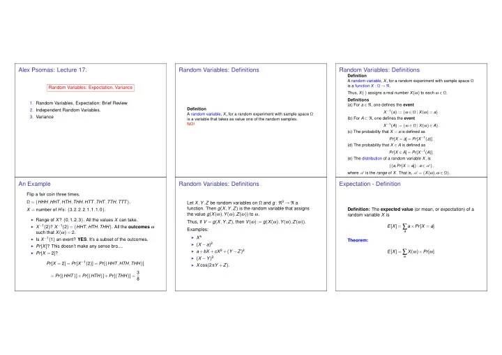
Alex Psomas: Lecture 17. Random Variables: Definitions Random Variables: Definitions Definition A random variable, X , for a random experiment with sample space Ω is a function X : Ω → ℜ . Random Variables: Expectation, Variance Thus, X ( · ) assigns a real number X ( ω ) to each ω ∈ Ω . Definitions 1. Random Variables, Expectation: Brief Review (a) For a ∈ ℜ , one defines the event Definition 2. Independent Random Variables. X − 1 ( a ) := { ω ∈ Ω | X ( ω ) = a } . A random variable, X , for a random experiment with sample space Ω 3. Variance (b) For A ⊂ ℜ , one defines the event is a variable that takes as value one of the random samples. NO! X − 1 ( A ) := { ω ∈ Ω | X ( ω ) ∈ A } . (c) The probability that X = a is defined as Pr [ X = a ] = Pr [ X − 1 ( a )] . (d) The probability that X ∈ A is defined as Pr [ X ∈ A ] = Pr [ X − 1 ( A )] . (e) The distribution of a random variable X , is { ( a , Pr [ X = a ]) : a ∈ A } , where A is the range of X . That is, A = { X ( ω ) , ω ∈ Ω } . An Example Random Variables: Definitions Expectation - Definition Flip a fair coin three times. Let X , Y , Z be random variables on Ω and g : ℜ 3 → ℜ a Ω = { HHH , HHT , HTH , THH , HTT , THT , TTH , TTT } . function. Then g ( X , Y , Z ) is the random variable that assigns X = number of H ’s: { 3 , 2 , 2 , 2 , 1 , 1 , 1 , 0 } . Definition: The expected value (or mean, or expectation) of a the value g ( X ( ω ) , Y ( ω ) , Z ( ω )) to ω . random variable X is ◮ Range of X ? { 0 , 1 , 2 , 3 } . All the values X can take. Thus, if V = g ( X , Y , Z ) , then V ( ω ) := g ( X ( ω ) , Y ( ω ) , Z ( ω )) . E [ X ] = ∑ ◮ X − 1 ( 2 ) ? X − 1 ( 2 ) = { HHT , HTH , THH } . All the outcomes ω a × Pr [ X = a ] . Examples: a such that X ( ω ) = 2. ◮ X k ◮ Is X − 1 ( 1 ) an event? YES . It’s a subset of the outcomes. Theorem: ◮ ( X − a ) 2 ◮ Pr [ X ] ? This doesn’t make any sense bro.... ◮ a + bX + cX 2 +( Y − Z ) 2 E [ X ] = ∑ X ( ω ) × Pr [ ω ] . ◮ Pr [ X = 2 ] ? ◮ ( X − Y ) 2 ω Pr [ X = 2 ] = Pr [ X − 1 ( 2 )] = Pr [ { HHT , HTH , THH } ] ◮ X cos ( 2 π Y + Z ) . = Pr [ { HHT } ]+ Pr [ { HTH } ]+ Pr [ { THH } ] = 3 8

An Example Win or Lose. Law of Large Numbers Expected winnings for heads/tails games, with 3 flips? An Illustration: Rolling Dice Recall the definition of the random variable X : { HHH , HHT , HTH , HTT , THH , THT , TTH , TTT } → { 3 , 1 , 1 , − 1 , 1 , − 1 , − 1 , − 3 } . Flip a fair coin three times. E [ X ] = 31 8 + 13 8 − 13 8 − 31 8 = 0 . Ω = { HHH , HHT , HTH , THH , HTT , THT , TTH , TTT } . X = number of H ’s: { 3 , 2 , 2 , 2 , 1 , 1 , 1 , 0 } . Thus, Can you ever win 0? X ( ω ) Pr [ ω ] = 31 8 + 21 8 + 21 8 + 21 8 + 11 8 + 11 8 + 11 8 + 01 Apparently: Expected value is not a common value. It doesn’t have to ∑ 8 . be in the range of X . ω The expected value of X is not the value that you expect! Also, It is the average value per experiment, if you perform the experiment a × Pr [ X = a ] = 31 8 + 23 8 + 13 8 + 01 ∑ 8 . many times. Let X 1 be your winnings the first time you play the game, a X 2 are your winnings the second time you play the game, and so on. (Notice that X i ’s have the same distribution!) When n ≫ 1 : X 1 + ··· + X n → 0 n The fact that this average converges to E [ X ] is a theorem: the Law of Large Numbers. (See later.) Indicators Linearity of Expectation Using Linearity - 1: Dots on dice Definition Theorem: Expectation is linear Roll a die n times. Let A be an event. The random variable X defined by X m = number of dots on roll m . E [ a 1 X 1 + ··· + a n X n ] = a 1 E [ X 1 ]+ ··· + a n E [ X n ] . � 1 , if ω ∈ A X = X 1 + ··· + X n = total number of dots in n rolls. X ( ω ) = 0 , if ω / ∈ A Proof: E [ X ] = E [ X 1 + ··· + X n ] is called the indicator of the event A . = E [ X 1 ]+ ··· + E [ X n ] , by linearity E [ a 1 X 1 + ··· + a n X n ] = ∑ = nE [ X 1 ] , because the X m have the same distribution Note that Pr [ X = 1 ] = Pr [ A ] and Pr [ X = 0 ] = 1 − Pr [ A ] . ( a 1 X 1 + ··· + a n X n )( ω ) Pr [ ω ] ω Hence, = ∑ Now, ( a 1 X 1 ( ω )+ ··· + a n X n ( ω )) Pr [ ω ] 6 = 6 × 7 E [ X 1 ] = 1 × 1 6 + ··· + 6 × 1 × 1 6 = 7 ω 2 . E [ X ] = 1 × Pr [ X = 1 ]+ 0 × Pr [ X = 0 ] = Pr [ A ] . 2 = a 1 ∑ X 1 ( ω ) Pr [ ω ]+ ··· + a n ∑ X n ( ω ) Pr [ ω ] ω ω This random variable X ( ω ) is sometimes written as = a 1 E [ X 1 ]+ ··· + a n E [ X n ] . Hence, E [ X ] = 7 n 2 . 1 { ω ∈ A } or 1 A ( ω ) . Note: If we had defined Y = a 1 X 1 + ··· + a n X n has had tried to Note: Computing ∑ x xPr [ X = x ] directly is not easy! compute E [ Y ] = ∑ y yPr [ Y = y ] , we would have been in trouble! Thus, we will write X = 1 A .

Y X Using Linearity - 2: Expected number of times a word Using Linearity - 2: Expected number of times a word Using Linearity - 3: The birthday paradox appears. appears. Let X be the random variable indicating the number of pairs of people, in a group of k people, sharing the same birthday. Alex is typing a document randomly: Each letter has a What’s E ( X ) ? 1 probability of 26 of being types. The document will be Let X i , j be the indicator random variable for the event that two 100,000,000 letters long. What is the expected number of times people i and j have the same birthday. X = ∑ i , j X i , j . that the word ”pizza” will appear? E ( X i ) = ( 1 26 ) 5 Let X be a random variable that counts the number of times the E [ X ] = E [ ∑ X i , j ] word ”pizza” appears. We want E ( X ) . i , j Therefore, E ( X ) = ∑ = ∑ E [ X i , j ] X ( ω ) Pr [ ω ] . E ( X i ) = 999 , 999 , 996 ( 1 26 ) 5 ≈ 84 X i ) = ∑ E ( X ) = E ( ∑ i , j ω i i = ∑ Better approach: Let X i be the indicator variable that takes Pr [ X i , j ] value 1 if ”pizza” starts on the i -th letter, and 0 otherwise. i i , j � 1 takes from 1 to 100 , 000 − 4 = 999 , 999 , 996. 1 � k 365 = k ( k − 1 ) 1 = ∑ 365 = hpizzafgnpizzadjgbidgne.... 2 2 365 i , j X 2 = 1, X 10 = 1,... For a group of 28 it’s about 1. For 100 it’s 13 . 5. For 280 it’s 107. Calculating E [ g ( X )] An Example Calculating E [ g ( X , Y , Z )] Let Y = g ( X ) . Assume that we know the distribution of X . Let X be uniform in {− 2 , − 1 , 0 , 1 , 2 , 3 } . We have seen that E [ g ( X )] = ∑ x g ( x ) Pr [ X = x ] . We want to calculate E [ Y ] . Let also g ( X ) = X 2 . Then (method 2) Using a similar derivation, one can show that Method 1: We calculate the distribution of Y : E [ g ( X , Y , Z )] = ∑ 3 g ( x , y , z ) Pr [ X = x , Y = y , Z = z ] . Pr [ Y = y ] = Pr [ X ∈ g − 1 ( y )] where g − 1 ( x ) = { x ∈ ℜ : g ( x ) = y } . x 2 1 ∑ E [ g ( X )] = x , y , z 6 This is typically rather tedious! x = − 2 An Example. Let X , Y be as shown below: { 4 + 1 + 0 + 1 + 4 + 9 } 1 6 = 19 Method 2: We use the following result. = 6 . Theorem: E [ g ( X )] = ∑ Method 1 - We find the distribution of Y = X 2 : g ( x ) Pr [ X = x ] . 0 . 2 0 . 3 1 x ∈ A ( X ) w.p. 2 8 (0 , 0) , w.p. 0 . 1  Proof: 4 , > > 6 (1 , 0) , w.p. 0 . 4 <  ( X , Y ) = w.p. 2  = ∑ g ( X ( ω )) Pr [ ω ] = ∑ 1 , (0 , 1) , w.p. 0 . 2  E [ g ( X )] ∑ g ( X ( ω )) Pr [ ω ] Y = 6 > > : (1 , 1) , w.p. 0 . 3 w.p. 1 0 , x ω ∈ X − 1 ( x ) ω 0 . 1 0 . 4 6  0  w.p. 1 = ∑ g ( x ) Pr [ ω ] = ∑  9 , 6 . ∑ g ( x ) ∑ Pr [ ω ] 0 1 x ω ∈ X − 1 ( x ) x ω ∈ X − 1 ( x ) E [ cos ( 2 π X + π Y )] = 0 . 1cos ( 0 )+ 0 . 4cos ( 2 π )+ 0 . 2cos ( π )+ 0 . 3cos ( 3 π ) = ∑ Thus, g ( x ) Pr [ X = x ] . E [ Y ] = 42 6 + 12 6 + 01 6 + 91 6 = 19 = 0 . 1 × 1 + 0 . 4 × 1 + 0 . 2 × ( − 1 )+ 0 . 3 × ( − 1 ) = 0 . x 6 .

X µ µ ⇔ X Center of Mass Best Guess: Least Squares Independent Random Variables. The expected value has a center of mass interpretation: Definition: Independence 0 . 5 0 . 5 0 . 7 0 . 3 The random variables X and Y are independent if and only if If you only know the distribution of X , it seems that E [ X ] is a 0 1 0 1 ‘good guess’ for X . Pr [ Y = b | X = a ] = Pr [ Y = b ] , for all a and b . 0 . 7 0 . 5 The following result makes that idea precise. p 1 p 2 p 3 p n ( a n − µ ) = 0 Fact: a 2 a 3 n Theorem a 1 = a n p n = E [ X ] The value of a that minimizes E [( X − a ) 2 ] is a = E [ X ] . X , Y are independent if and only if p 1 ( a 1 − µ ) n p 3 ( a 3 − µ ) p 2 ( a 2 − µ ) Unfortunately, we won’t talk about this in this class... Pr [ X = a , Y = b ] = Pr [ X = a ] Pr [ Y = b ] , for all a and b . Obvious. Independence: Examples Functions of Independent random Variables Mean of product of independent RV Theorem Let X , Y be independent RVs. Then Example 1 E [ XY ] = E [ X ] E [ Y ] . Roll two die. X = number of dots on the first one, Y = number Theorem Functions of independent RVs are independent of dots on the other one. X , Y are independent. Let X , Y be independent RV. Then Proof: Indeed: Pr [ X = a , Y = b ] = 1 36 , Pr [ X = a ] = Pr [ Y = b ] = 1 6 . Recall that E [ g ( X , Y )] = ∑ x , y g ( x , y ) Pr [ X = x , Y = y ] . Hence, f ( X ) and g ( Y ) are independent, for all f ( · ) , g ( · ) . Example 2 = ∑ xyPr [ X = x , Y = y ] = ∑ E [ XY ] xyPr [ X = x ] Pr [ Y = y ] , by ind. Roll two die. X = total number of dots, Y = number of dots on x , y x , y die 1 minus number on die 2. X and Y are not independent. = ∑ xyPr [ X = x ] Pr [ Y = y ]] = ∑ [ ∑ [ xPr [ X = x ]( ∑ yPr [ Y = y ])] Indeed: Pr [ X = 12 , Y = 1 ] = 0 � = Pr [ X = 12 ] Pr [ Y = 1 ] > 0. x y x y = ∑ [ xPr [ X = x ] E [ Y ]] = E [ X ] E [ Y ] . x