Ray Tracing Recursive rays Reflection Refraction Thanks to - - PDF document

1

Ray Tracing

Thanks to UDel and MIT

Outline

• Recursive rays

– Reflection – Refraction

Ray Tracing

• Model: Perceived color at point p is an additive combination of local

illumination (e.g., Phong), reflection, and refraction effects

• Compute reflection, refraction contributions by tracing respective

rays back from p to surfaces they came from and evaluating local illumination at those locations

• Apply operation recursively to some maximum depth to get:

– Reflections of reflections of ... – Refractions of refractions of ... – And of course mixtures of the two

from Hill

Reflections

incident ray v reflected ray r

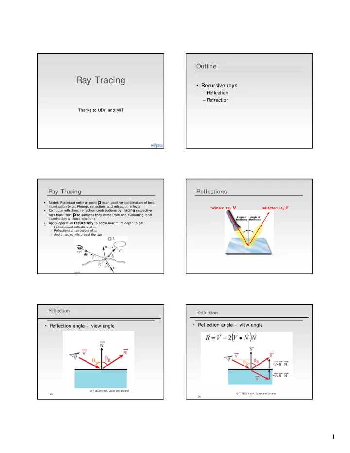
Reflection

• Reflection angle = view angle

MIT EECS 6.837, Cutler and Durand 25

Reflection

• Reflection angle = view angle

MIT EECS 6.837, Cutler and Durand 26

2

Mirror Reflection

• Compute mirror contribution
• Cast ray

–In direction symmetric wrtnormal

• Multiply by reflection coefficient (color)

MIT EECS 6.837, Cutler and Durand 23

Mirror Reflection

• Cast ray

–In direction symmetric wrtnormal

• Don’t forget to add epsilon

to the ray Without epsilon With epsilon

MIT EECS 6.837, Cutler and Durand 24

Amount of Reflection

• Traditional (hacky) ray tracing

–Constant coefficient

reflectionColor –Component per component multiplication

MIT EECS 6.837, Cutler and Durand 27

Amount of Reflection

• More realistic:

–Fresnelreflection term –More reflection at grazing angle –Schlick’sapproximation: R(θ)= R0+ (1-R0)(1-cos θ)5

MIT EECS 6.837, Cutler and Durand 28

Example: Reflections at depth = 0

3

Example: Reflections at depth = 1 Example: Reflections at depth = 2 Example: Reflections at depth = 3

Transparency

• Compute transmitted contribution
• Cast ray

–In refracted direction

• Multiply by transparency coefficient (color)

31

Qualitative refraction

• From “Color and Light in Nature” by Lynch and Livingston

MIT EECS 6.837, Cutler and Durand 32

Refraction

Snell-Descartes Law

ni sini = nt sint

MATERIAL INDEX OF REFRACTION air/vacuum 1 water 1.33 glass about 1.5 diamond 2.4

Note that I is the negative

• f the incoming ray

MIT EECS 6.837, Cutler and Durand 33

4

Refraction Snell-Descartes Law

Note that I is the negative

• f the incoming ray

MIT EECS 6.837, Cutler and Durand 34

ni sini = nt sint

Refraction Snell-Descartes Law

Note that I is the negative of the incoming ray

MIT EECS 6.837, Cutler and Durand 35

Refraction

Snell-Descartes Law

Note that I is the negative of the incoming ray

MIT EECS 6.837, Cutler and Durand 36

Refraction

MIT EECS 6.837, Cutler and Durand 37

Use: sin2 + cos2 = 1

Refraction

MIT EECS 6.837, Cutler and Durand 38

Total internal reflection

• From “Color and Light in Nature” by Lynch and

Livingstone

MIT EECS 6.837, Cutler and Durand 39

5

Example: Refraction

Ray Tracing Example (with texture mapping)

courtesy of J. Lee

Refraction and the lifeguard problem

• Running is faster than swimming

MIT EECS 6.837, Cutler and Durand 42

The Ray Tree

Ni surface normal Ri reflected ray Li shadow ray Ti transmitted (refracted) ray

MIT EECS 6.837, Cutler and Durand 51

Ray Tree

Draw the ray-tree to depth 3 for the following initial ray (boxes are solid plastic, sphere is glass): N

Basic Ray Tracing: Notes

• Intersection calculations are expensive, and

even more so for more complex objects

– Not currently suitable for real-time (i.e., games)

• Only global illumination effect is purely

specular reflection/transmission

– No “diffuse reflection” from other objects ! Still using ambient term – One remedy is radiosity (slow, offline, precompute – Ambient Occlusion

• Shadows have sharp edges, which is

unrealistic – next lecture

6

Phong shading Ambient Occlusion Ambient Occlusion Ambient Occlusion Ambient Occlusion Ray Tracing: Improvements

• Image quality: Anti-aliasing

– Supersampling: Shoot multiple rays per pixel (grid

• r jittered)
• Adaptive: More rays in areas where image is changing

more quickly

• Efficiency: Bounding extents

– Idea: Enclose complex objects in shapes (e.g., sphere, box) that are less expensive to test for intersection – Next lecture

7

Supersampling

• Rasterize at higher resolution

– Regular grid pattern around each “normal” image pixel – Irregular jittered sampling pattern reduces artifacts

• Combine multiple samples into
• ne pixel via weighted average

– “Box” filter: All samples associated with a pixel have equal weight (i.e., directly take their average) – Gaussian/cone filter: Sample weights inversely proportional to distance from associated pixel

from Hill

Regular supersampling with 2x frequency Jittered supersampling

Adaptive Supersampling (Whitted’s method)

• Shoot rays through 4 pixel corners

and collect colors

• Provisional color for entire pixel is

average of corner contributions

– If you stop here, the only overhead

• vs. center-of-pixel ray-tracing is

another row, column of rays

• If any corner’s color is too

different, subdivide pixel into quadrants and recurse on quadrants

from Hill

Adaptive Supersampling: Details

OK Must subdivide