Introduction to Path Tracing Marc Sunet Table of contents From Ray - PowerPoint PPT Presentation
Introduction to Path Tracing Marc Sunet Table of contents From Ray Tracing to Path Tracing The Rendering Equation Monte Carlo Integration A Basic Path Tracer Variance Reduction and Optimisation Techniques Additional Resources Plan From Ray
Introduction to Path Tracing Marc Sunet
Table of contents From Ray Tracing to Path Tracing The Rendering Equation Monte Carlo Integration A Basic Path Tracer Variance Reduction and Optimisation Techniques Additional Resources
Plan From Ray Tracing to Path Tracing The Rendering Equation Monte Carlo Integration A Basic Path Tracer Variance Reduction and Optimisation Techniques Additional Resources
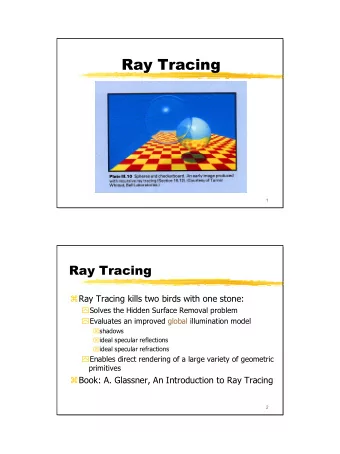
Ray Tracing ◮ Ray tracing is a rendering technique that generates images by tracing rays through each pixel and simulating the interaction of light with the objects in a scene.
Whitted Ray Tracing ◮ First recursive ray tracer by Turner Whitted (1979). ◮ Simulates (perfect specular) reflections, refractions and (hard) shadows.
Whitted Ray Tracing render image ( ) : f o r each p i x e l : ray = camera ray ( p i x e l ) c o l o u r = t r a c e ( ray ) t r a c e ( ray ) : point , normal = i n t e r s e c t ( ray , scene ) c o l o u r = shade ( point , normal ) shade ( point , normal ) : c o l o u r = 0 f o r each l i g h t source : t r a c e shadow ray to l i g h t source i f i n t e r s e c t s ( shadow ray , l i g h t source ) c o l o u r = c o l o u r + d i r e c t i l l u m i n a t i o n i f s p e c u l a r : c o l o u r = c o l o u r + t r a c e ( r e f l e c t e d / r e f r a c t e d ray )
Whitted Ray Tracing Limitations: ◮ No indirect illumination in diffuse surfaces. ◮ Hard shadows only. ◮ No glossy surfaces. ◮ No subsurface scattering. ◮ No participating media. ◮ No focusing effects due to camera lens. ◮ No motion blur. ◮ etc. Whitted ray tracing is not a full global illumination algorithm.
Path Tracing https://www . youtube . com/watch?v=abqAanC2NZs Brigade
Path Tracing ◮ Generalisation of the original ray tracing algorithm. ◮ Full global illumination light transport algorithm. ◮ Stochastically samples all light paths to simulate all light/scene interactions. ◮ Algorithm is unbiased 1 if implemented carefully. Buzzword definition to impress friends & family: ”Mathematically, path tracing is a continuous Markov chain random walk technique for solving the rendering equation. The solution technique can be seen as a Monte Carlo sampling of the Neumann series expansion of the rendering equation.” — [Realistic Image Synthesis Using Photon Mapping] 1 https://en . wikipedia . org/wiki/Bias of an estimator
Plan From Ray Tracing to Path Tracing The Rendering Equation Monte Carlo Integration A Basic Path Tracer Variance Reduction and Optimisation Techniques Additional Resources
Light Reflection Before delving into the path tracing algorithm, we need to understand what are we actually trying to compute. Goal: generate an image of the scene being viewed. ◮ Viewer sees point x through a given pixel. ◮ Light reflected at x towards viewer depends on light incident at x from all directions in the normal-oriented hemisphere. ◮ Reflected light also depends on the properties of the surface.
Light Reflection To compute light reflected towards viewer, we therefore need two ingredients: ◮ Determine the light incident at x from all directions in the hemisphere → ray tracing . ◮ Determine the properties of the surface, which describe how incident light is reflected → BRDF 2 . 2 Although more general light reflection models exist, we will focus on the BRDF to keep it simple.
The BRDF Q : How much light is reflected at point p in direction ω o due to light coming in direction ω i ? A : BRDF f(p, ω o , ω i ) The BRDF describes how light reflects off a surface.
Common BRDFs Specular reflects light in a single direction - the direction of mirror reflection. Diffuse reflects light equally in all directions. Glossy reflects light in a cone centered in the direction of mirror reflection.
The Rendering Equation Determines outgoing radiance as a function of incoming radiance and surface BRDF. � L o ( p , ω o ) = f ( p , ω o , ω i ) L i ( p , ω i ) cos θ i d ω i Ω L o ( p , ω o ) total outgoing radiance reflected at p in direction ω o . L i ( p , ω i ) radiance incident at p in direction ω i . f ( p , ω o , ω i ) determines how much radiance is reflected at p in direction ω o due to irradiance incident at p in direction ω i . 3 cos θ i Lambert’s cosine law. 3 For a full definition, see the BRDF section on Wikipedia.
Plan From Ray Tracing to Path Tracing The Rendering Equation Monte Carlo Integration A Basic Path Tracer Variance Reduction and Optimisation Techniques Additional Resources
Monte Carlo Integration To compute the light that is reflected off a surface, we need to find a solution to the rendering equation. An analytical solution does not generally exist, so we rely on methods that approximate the integral numerically. Several methods exist to this end. However, we will focus solely on Monte Carlo integration .
Monte Carlo Integration A technique for numerical integration that uses random numbers. Pros ◮ Flexible and easy to implement: just need to evaluate the integrand at arbitrary points in order to evaluate the value of the integral. ◮ The convergence rate is independent of the number of dimensions in the integral. Monte Carlo integration does not suffer from the curse of dimensionality, where convergence rate grows exponentially with the number of dimensions. ◮ The number of samples is arbitrary; it does not depend on the dimensions of the integral. Cons 1 ◮ Variance is proportional to N , where N is the number of samples, √ i.e. if you want to reduce variance by half, you need to quadruple the number of samples.
Monte Carlo Integration Given � b I = f ( x ) d x a evaluate integral by taking the average value of f ( x ) along the interval [ a , b ] and multiply by the length of the interval b − a : average f ( x ) a b
Monte Carlo Integration To find the average value of f ( x ), evaluate f ( x ) at N different locations X 1 . . . X N , where X 1 . . . X N are uniformly distributed random numbers in the interval [ a , b ]: N f ( x ) = 1 ¯ � f ( X i ) N i =1 a b
Monte Carlo Estimator The average value of f ( x ) multiplied by the length of the interval b − a gives us the Monte Carlo estimator: N F N = b − a � f ( X i ) N i =1 In the limit, as we gather more and more samples, the Monte Carlo estimator takes on the value of the integral: � b N →∞ F N = lim f ( x ) d x a
Monte Carlo Integration: Two Interpretations
Monte Carlo Estimator: Proof The expected value of the Monte Carlo estimator is equal to the integral: � b E [ F N ] = f ( x ) d x a Proof Since X 1 . . . X N are uniformly distributed, their pdf p ( x ) must be equal to 1 b − a . Then...
Monte Carlo Estimator: Proof � N � b − a � E [ F N ] = E f ( X i ) N i =1 N = b − a � E [ f ( X i )] N i =1 � b N = b − a � f ( x ) p ( x ) d x N a i =1 � b N = 1 � f ( x ) d x N a i =1 � b = f ( x ) d x a
Monte Carlo Estimator: Generalised Version The cool part about Monte Carlo integration is that the random variables X i need not actually follow a uniform distribution. Monte Carlo integration works with any arbitrary pdf as long as the variables are independent and identically distributed (i.i.d). Given X 1 . . . X N distributed according to pdf p ( x ), the generalised Monte Carlo estimator is given by: N F N = 1 f ( X i ) � N p ( X i ) i =1 Again, the expected value of the estimator is the value of the integral: � b E [ F N ] = f ( x ) d x a
Monte Carlo Estimator: Proof Proof � N � 1 f ( X i ) � E [ F N ] = E N p ( X i ) i =1 N = 1 � f ( X i ) � � E N p ( X i ) i =1 � b N = 1 f ( x ) � p ( x ) p ( x ) d x N a i =1 � b N = 1 � f ( x ) d x N a i =1 � b = f ( x ) d x a
Importance Sampling Having the freedom to choose any arbitrary pdf p ( x ) is very useful in path tracing. Importance sampling allows us to better approximate the integral by choosing an appropriate pdf. The idea is to choose a pdf p ( x ) that is similar to the function being integrated f ( x ): p ( x ) ∼ f ( x ) It can be shown that using importance sampling results in faster convergence than using an arbitrary pdf. We will re-visit this concept later with specific examples.
Plan From Ray Tracing to Path Tracing The Rendering Equation Monte Carlo Integration A Basic Path Tracer Variance Reduction and Optimisation Techniques Additional Resources
Path Tracing 101 Rendering equation: � L o ( p , ω o ) = f ( p , ω o , ω i ) L i ( p , ω i ) cos θ i d ω i Ω Monte Carlo estimator: N F N = 1 f ( X i ) � N p ( X i ) i =1 Monte Carlo path tracing: N � L o ( p , ω o ) � = 1 f ( p , ω o , ω i ) L i ( p , ω i ) cos θ i � N p ( ω i ) i =1
Path Tracing 101 ◮ For every pixel, distribute N samples in that pixel. ◮ For every sample, generate a ray and trace a random path in the scene by randomly bouncing the ray around. ◮ For every bounce, compute the incoming radiance along the randomly reflected/refracted ray, weigh the result by the BRDF and divide by the pdf. ◮ Stop the recursion when you reach a maximum number of bounces or hit an emissive surface / light. ◮ Average the results of the N samples to produce the pixel’s final colour.
Recommend
More recommend
Explore More Topics
Stay informed with curated content and fresh updates.
