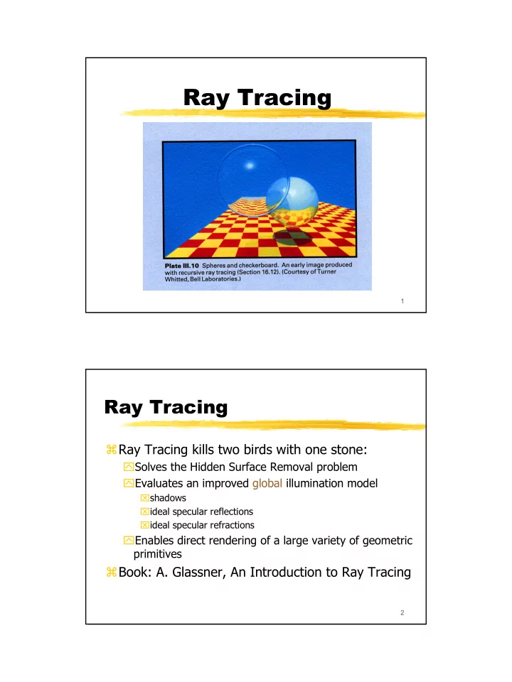
Ray Tracing 1 Ray Tracing Ray Tracing kills two birds with one - PDF document

Ray Tracing 1 Ray Tracing � Ray Tracing kills two birds with one stone: � Solves the Hidden Surface Removal problem � Evaluates an improved global illumination model ⌧ shadows ⌧ ideal specular reflections ⌧ ideal specular refractions � Enables direct rendering of a large variety of geometric primitives � Book: A. Glassner, An Introduction to Ray Tracing 2

Backward Tracing 3 Reflected, Transmitted and Shadow rays 4

The Illumination Model � Remember the local illumination model we saw earlier? � ∑ ( ) ( )   n = + ⋅ + ⋅ I I k f I k N L k R V   r a a att p d i s i i i = i 1 � First, let’s add shadows into the model: [ ] � ∑ ( ) ( ) = + ⋅ + ⋅ n I I k S f I k N L k R V r a a i att p d i s i i i = i 1 5 Illumination Model (cont’d) � Add in light arriving from the mirror- reflected direction k s I s � Add in light arriving from the ideal refracted direction (Snell’s Law) k t I t [ ] � ∑ ( ) ( ) n = + ⋅ + ⋅ I I k S f I k N L k R V r a a i att p d i s i i i = i 1 + + k I k I s s t t 6

Refraction 7 Refraction Geometry 8

And the result is... 9 10

11 12

The RT Algorithm � For each pixel (x,y) in the image, generate the corresponding ray in 3D. � Image(x,y) := TraceRay(ray) � TraceRay(ray) � compute nearest ray-surface intersection � if none found, return background color � compute direct illumination � compute illumination arriving from reflected direction � compute illumination arriving from refracted direction � combine illumination components using the shading model � return resulting color 13 The RT Algorithm � Direct illumination: test the visibility of each source by shooting a shadow ray towards it. Only sources which are found visible are summed in the shading model. � Reflected/refracted illumination: a recursive call to TraceRay with the reflected/refracted ray as argument. 14

The depth of reflection 15 Ray-Surface Intersection � Implicit surfaces: = f ( x , y , z ) 0 � Use a parametric representation for the ray: = + R t ( ) O tD = + R t ( ) O tD x x x R t ( ) = O + tD y y y = + R t ( ) O tD z z z � Substitute into the implicit equation: + + + = f ( O tD , O tD , O tD ) 0 x x y y z z � Solve the resulting equation � Examples: plane, sphere 16

Ray Plane intersection Implicit Formulation � Find ‘t’ such that f(x,y,z) = 0 = + R ( t ) O tD O = + R ( t ) O tD N x x x D = + R ( t ) O tD y y y = + R ( t ) O tD z z z = + + + = f x y z ( , , ) N x N y N z d 0 x y z + + + + + = − N O ( tD ) N ( O tD ) N O ( tD ) d x x x y y y z z z + + = − + + + ( N D N D N D t ) ( d N O N O N O ) x x y y z z x x y y z z + + + d N O N O N O = − x x y y z z t + + N D N D N D x x y y z z 17 Ray Sphere intersection � Find ‘t’ such that f(x,y,z) = 0 = + R t ( ) O tD O D = 2 + 2 + 2 − f x y z ( , , ) x y z 1 + + + + + = ( O tD ) 2 ( O tD ) 2 ( O tD ) 2 1 x x y y z z R ... C 18

Ray-Surface Intersection  x ( u , v )  � Parametric surfaces:   = S ( u , v ) y ( u , v )   � Several approaches:   z ( u , v )   � Tessellation � Subdivision � Implicitization � Other numerical methods (involve solving a system of two or three nonlinear equations) 19 Ray-Plane Intersection Explicit formulation � Find t, u,v such that: +  O tD   x u v ( , )   x u v ( , )   x u v ( , )   x  x x u v o           + = = + + O tD y u v ( , ) u y u v ( , ) v y u v ( , ) y           y y u v o  +          O tD z u v ( , ) z u v ( , ) z u v ( , ) z           z z u v o � Linear system 3 equations, 3 unknowns 20

Advantages of Ray Tracing Algorithm � Computes global illuminations effects: � Shadows � Reflections � Refractions � Computes visibility and shading at once � Consistent and easy implementation � Can be extended easily � Can be parallelized 21 Disadvantages of Ray Tracing � Slow � Memory bound – all objects must be kept in memory � Does not compute all global illuminations effects: � Caustics � Color Bleeding � More… 22

Accelerating Ray Tracing � Four main groups of acceleration techniques: � Parallelization, specialized hardware � Reducing the total number of rays that are traced ⌧ Adaptive recursion depth control � Reducing the average cost of intersecting a ray with a scene: ⌧ Faster intersection calculations ⌧ Fewer intersection calculations � Using generalized rays ⌧ beams ⌧ cones ⌧ pencils 23 Parallel/Distributed RT � Two main approaches: � Each processor is in charge of tracing a subset of the rays. Requires a shared memory architecture, replication of the scene database, or transmission of objects between processors on demand. � Each processor is in charge of a subset of the scene (either in terms of space, or in terms of objects). Requires processors to transmit rays among themselves. 24

The Ray Tree 25 Accelerating Ray Tracing � Faster intersection calculations: � Object-dependent optimizations � Bounding volumes � Fewer intersection calculations: � Bounding volume hierarchy � Spatial subdivisions: ⌧ Uniform grids ⌧ Octrees ⌧ BSP-trees ⌧ Hybrids � Directional techniques ⌧ The light buffer ⌧ Ray classification 26

Bounding Volumes � Idea: associate with each object a simple bounding volume. If a ray misses the bounding volume, it also misses the object contained therein. � Common bounding volumes: � spheres � bounding boxes � bounding slabs � Effective for additional applications: � Clipping acceleration � Collision detection � Note: bounding volumes offer no asymptotic improvement! 27 Bounding Boxes 28

Bounding Volumes 29 Bounding Volume Hierarchy � Introduced by James Clark (SGI, Netscape) in 1976 for efficient view-frustum culling. Procedure IntersectBVH(ray Procedure IntersectBVH(ray, node) , node) begin begin if if IsLeaf(node IsLeaf(node) ) then then Intersect(ray, node.object) Intersect(ray, node.object) else if IntersectBV(ray,node.boundingVolume IntersectBV(ray,node.boundingVolume) ) else if then then foreach child of node do foreach child of node do IntersectBVH(ray IntersectBVH(ray, child) , child) endfor endfor endif endif end end 30

Spatial Subdivision � Uniform spatial subdivision: � The space containing the scene is subdivided into a uniform grid of cubes “voxels”. � Each voxel stores a list of all objects at least partially contained in it.in � Given a ray, voxels are traversed using a 3D variant of the 2D line drawing algorithms. � At each voxel the ray is tested for intersection with the primitives stored therein � Once an intersection has been found, there is no need to continue to other voxels. 31 Uniform Subdivision 32

Adaptive Spatial Subdivision � Disadvantages of uniform subdivision: � requires a lot of space � traversal of empty regions of space can be slow � not suitable for “teapot in a stadium” scenes � Solution: use a hierarchical adaptive spatial subdivision data structure � octrees � BSP-trees � Given a ray, perform a depth-first 33 traversal of the tree Again can stop once Octrees 34

Octree traversal 35 Directional Techniques � Light buffer: accelerates shadow rays. � Discretize the space of directions around each light source using the direction cube � In each cell of the cube store a sorted list of objects visible from the light source through that cell � Given a shadow ray locate the appropriate cell of the direction cube and test the ray with the objects on its list 36

Directional Techniques � Ray classification (Arvo and Kirk 87): � Rays in 3D have 5 degrees of freedom: (x,y,z, θ,φ ) � Rays coherence: rays belonging to the same small 5D neighborhood are likely to intersect the same set of objects. � Partition the 5D space of rays into a collection of 5D hypercubes, each containing a list of objects. � Given a ray, find the smallest containing 5D hypercube, and test the ray against the objects on the list. � For efficiency, the hypercubes are arranged in a hierarchy: a 5D analog of the 3D octree. This data structure is constructed in a lazy fashion. 37