[PPT] - Random Variables Overview Taylor Series Expansion Probability PowerPoint Presentation

SLIDE 1

Introduction

Random signals evolve in time in an unpredictable manner
We must assume something doesn’t change in order to use them
Usually this is their average properties
J. McNames

Portland State University ECE 538/638 Random Variables

Ver. 1.07

3

Random Variables Overview

Probability
Random variables
Transforms of pdfs
Moments and cumulants
Useful distributions
Random vectors
Linear transformations of random vectors
The multivariate normal distribution
Sums of independent random variables
Central limit theorem
J. McNames

Portland State University ECE 538/638 Random Variables

Ver. 1.07

1

Probability Space

Let Ω denote all possible outcomes, ζ, of an experiment
Event: A subset of outcomes
The event is said to occur if the outcome of the experiment is one
f the members of the subset

– It’s an “or” (union) – Not an “and” (intersection)

A collection of subsets with certain properties is called a field and

will be denoted as F

The probability of each event in the field is denoted Pr {·} for

k = 1, 2, . . .

The collection (Ω, F, Pr {·}) is called a probability space
J. McNames

Portland State University ECE 538/638 Random Variables

Ver. 1.07

4

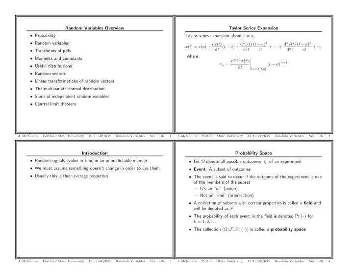
Taylor Series Expansion Taylor series expansion about t = a,

x(t) = x(a) + dx(t) dt (t − a) + d2x(t) d2t (t − a)2 2! + · · · + dnx(t) dnt (t − a)n n! + rn

where rn = dn+1x(t) dt

t=τ∈[t,a]

(t − a)n+1

J. McNames

Portland State University ECE 538/638 Random Variables

Ver. 1.07

2

SLIDE 2

Random Variable Properties Continued

Notation: x(ζ) = x

– x(ζ) denotes a random variable (function of the experimental

utcome)

– x denotes its value

A random variable may be Discrete-Valued,

Continuous-Valued, or Mixed

Similar to spectral densities

– If x(t) is nearly periodic, it has discrete spectra – Most stationary random signals x(t) have continuous spectra – A combination of the two types has mixed spectra

J. McNames

Portland State University ECE 538/638 Random Variables

Ver. 1.07

7

Random Variables

Real Line Range

x(ζ) ζ Ω

Random variable: a function that assigns a real number, x(ζ), to

each outcome ζ in the sample space of a random experiment

Conditions

– {ζ : ζ ∈ Ω and − ∞ < x(ζ) ≤ x0} ∈ F for all x0 ∈ R1 – Pr {x(ζ) = ∞} = 0 – Pr {x(ζ) = −∞} = 0

J. McNames

Portland State University ECE 538/638 Random Variables

Ver. 1.07

5

Cumulative Distribution Function (cdf)

Recall that probability is defined on the field of possible events
Some of these events (subsets of outcomes) can be defined as

{ζ : x(ζ) ≤ x}

Cumulative Distribution Function (cdf): The probability of

these events, Pr {x(ζ) ≤ x}

Note the cdf is a function of x ∈ R1:

Fx(x) Pr {x(ζ) ≤ x}

The cdf is continuous from the right
J. McNames

Portland State University ECE 538/638 Random Variables

Ver. 1.07

8

Random Variable Properties

The sample space Ω is the domain of the random variable
The set of all values that x(·) can have is the range of the

random variable

For now the range is the real line, R1
Later we will generalize to allow it to be a vector or a sequence
This is a many to one mapping. That is, a set of points, ζ1, ζ2, . . .

may take on the same value of the random variable

Will sometimes abbreviate RV
The RV may be real- or complex-valued
Random variables are actually a deterministic function of any

event in the field: {ζ1, ζ2, . . . , ζk}

J. McNames

Portland State University ECE 538/638 Random Variables

Ver. 1.07

6

SLIDE 3

Properties of the pdf

fx(x) ≥ 0
Pr {a ≤ x(ζ) ≤ b} =

b

a fx(u) du

Fx(x) =

x

−∞ fx(u) du

+∞

−∞ fx(u) du = 1

A valid pdf can be formed from any nonnegative, piecewise

continuous function g(x) that has a finite integral

The pdf must be defined for all real values of x
If x does not take on some values, this implies fx(x) = 0 for those

values

J. McNames

Portland State University ECE 538/638 Random Variables

Ver. 1.07

11

Properties of the cdf

0 ≤ Fx(x) ≤ 1
limx→+∞ Fx(x) = 1
limx→−∞ Fx(x) = 0
Fx(x) is a nondecreasing function of x

– Thus, if a < b, then Fx(a) ≤ Fx(b)

Fx(x) is continuous from the right

– That is, for h > 0, Fx(b) = limh→0 Fx(b + h) = Fx(b+)

Pr {a < x(ζ) ≤ b} = Fx(b) − Fx(a)
Pr {x(ζ) = b} = Fx(b) − Fx(b−)
J. McNames

Portland State University ECE 538/638 Random Variables

Ver. 1.07

9

Point Statistics, Averages, and Moments

In general, we will often not have a complete description of an RV

(the pdf or cdf)

Estimating a pdf or cdf is difficult in general, especially if x(ζ) is a

sequence or vector

However, we can often estimate some properties of the

distribution without estimating the distribution itself

These are called point statistics
We will only discuss a subset of point statistics: statistical

averages or moments

These are useful because

– In many cases, we can estimate them accurately from data – They give us useful information about the distribution – We don’t have to know the distribution to estimate them

J. McNames

Portland State University ECE 538/638 Random Variables

Ver. 1.07

12

Probability Density Function (pdf)

Probability Density Function (pdf): When it exists, is defined

as fx(x) dFx(x) dx

Thus, we also have

Fx(x) = x

−∞

fx(u) du

For a small interval △x, can be thought of as

fx(x)△x ≈ Fx(x + △x) − Fx(x) = Pr {x < x(ζ) ≤ x + △x}

J. McNames

Portland State University ECE 538/638 Random Variables

Ver. 1.07

10

SLIDE 4

Moments Defined mth-order Moment of x(ζ) is defined as r(m)

x

E [xm(ζ)] = ∞

−∞

xmfx(x) dx mth-order Central Moment of x(ζ) is defined as γ(m)

x

E [(x(ζ) − µx)m] = ∞

−∞

(x − µx)mfx(x) dx

Mean-Squared Value: The second-order moment, r(2)

x .

Note that

E

x2(ζ)
= E2 [x(ζ)]
J. McNames

Portland State University ECE 538/638 Random Variables

Ver. 1.07

15

Expected Values Defined Expected value: defined for a random variable x(ζ) as E[x(ζ)] µx = +∞

−∞

xfx(x) dx If x(ζ) is discrete-valued, the pdf consists only of impulses and can be alternatively written in terms of the pmf E [x(ζ)] = +∞

−∞

x

k

pkδ(x − xk)

dx

=

k

pk +∞

−∞

xδ(x − xk) dx =

k

pkxk

J. McNames

Portland State University ECE 538/638 Random Variables

Ver. 1.07

13

Moments and Definitions r(m)

x

E [xm(ζ)] =

∞

−∞

xmfx(x) dx γ(m)

x

E [(x(ζ) − µx)m] =

∞

−∞

(x − µx)mfx(x) dx

Variance of x(ζ) is defined as

var[x(ζ)] σ2

x γ(2) x

= E

(x(ζ) − µx)2
Standard deviation of x(ζ) is defined as σx =
var[x(ζ)]
Obvious moments

r(0)

x

= 1 r(1)

x

= µx

Trivial central moments

γ(0)

x

= 1 γ(1)

x

= 0 γ(2)

x

= σ2

x

J. McNames

Portland State University ECE 538/638 Random Variables

Ver. 1.07

16

Expectation Properties E [x(ζ)] µx = +∞

−∞

xfx(x) dx

Also called the mean of x(ζ)
The mean can be regarded as the “center of gravity” of fx(x)
If fx(x) is symmetric about a, f(x − a) = f(a − x), then µx = a
If fx(x) is even, µx = 0
This is a linear operation

E [αx(ζ) + β] = αµx + β

If y(ζ) = g(x(ζ)), a function of the random variable x(ζ), y(ζ) is

also a random variable such that E [y(ζ)] E [g(x(ζ))] = ∞

−∞

g(x)fx(x) dx

J. McNames

Portland State University ECE 538/638 Random Variables

Ver. 1.07

14

SLIDE 5

Moment Generating Functions Moment Generating Function of x(ζ) is defined as ¯ Φ(s) E

esx(ζ)

= ∞

−∞

fx(x)esx dx

Similar to the continuous-time Laplace transform
However, the exponent is positive (why?)

Using a Taylor series expansion of esx at x close to zero we have ¯ Φ(s) = E

esx(ζ)

= E

1 + sx(ζ) + [sx(ζ)]2

2! + · · · + [sx(ζ)]m m! + . . .

=

1 + sµx + s2 2! r(2)

x

+ · · · + sm m! r(m)

x

+ . . .

J. McNames

Portland State University ECE 538/638 Random Variables

Ver. 1.07

19

Relationship of Moments Moments and central moments are related: γ(m)

x

=

m

k=0

m k

(−1)kµk

xr(m−k) x

It also possible to calculate the first m moments from the first m central moments.

J. McNames

Portland State University ECE 538/638 Random Variables

Ver. 1.07

17

Moment Generating Functions ¯ Φ(s) = 1 + sµx + s2 2! r(2)

x

+ · · · + sm m! r(m)

x

+ . . .

If all the moments of x(ζ) are known and exist, we can create

¯ Φ(s) and solve for fx(x) by inverse Laplace transform

Thus the set of all moments (if they exist) completely define the

pdf!

If ¯

Φ(s) is known and analytic (not in the book), we can use it to solve for the moments r(m)

x

= dm[¯ Φ(s)] dsm

s=0

= (−j)m dm[¯ Φ(ξ)] dξm

ξ=0
J. McNames

Portland State University ECE 538/638 Random Variables

Ver. 1.07

20

Characteristic Functions Characteristic Function of x(ζ) is defined as Φ(ξ) E

ejξx(ζ)

= ∞

−∞

fx(x)ejξx dx

Similar to the continuous-time Fourier transform
However, the exponent is positive (why?)
Will not use Fx(ξ) to avoid confusion with cdf (same as text)
Text claims the independent variable ξ should not be thought of

as frequency (why?)

This will be useful for handling sums of random variables because

the distribution of the sum is the convolution of the pdf’s

J. McNames

Portland State University ECE 538/638 Random Variables

Ver. 1.07

18

SLIDE 6

Uniform Distribution fx(x) =

1

b−a

a ≤ x ≤ b

therwise
Useful for situations in which outcomes are equally likely
Often denoted as x(ζ) ∼ U[a, b]
Mean and variance

µx = a + b 2 σ2

x = (b − a)2

12

J. McNames

Portland State University ECE 538/638 Random Variables

Ver. 1.07

23

Cumulants Cumulant Generating Function of x(ζ) is defined as ¯ Ψx(s) ln ¯ Φx(s) = ln E

esx(ζ)

Second Characteristic Function of x(ζ) is defined as Ψx(ξ) ln Φx(ξ) = ln E

ejξx(ζ)

mth Cumulant of x(ζ) is defined as κ(m)

x

dm[¯ Ψ(s)] dsm

s=0

= (−j)m dm[¯ Ψ(ξ)] dξm

ξ=0

Useful for high-order moment analysis (advanced SSP topic) and working with products of characteristic functions

J. McNames

Portland State University ECE 538/638 Random Variables

Ver. 1.07

21

Normal Distribution

−5 −4 −3 −2 −1 1 2 3 4 5 0.2 0.4 0.6 0.8 1 x F(x) Gaussian Distribution Function −5 −4 −3 −2 −1 1 2 3 4 5 0.1 0.2 0.3 0.4 x f(x) Gaussian Density Function

fx(x) = 1

2πσ2

x

exp

−(x − µx)2

2σ2

x

Also called the Gaussian distribution
Often denoted as x(ζ) ∼ N(µx, σ2

x)

Arises naturally in many applications
Central limit theorem (more later)
J. McNames

Portland State University ECE 538/638 Random Variables

Ver. 1.07

24

Common Random Variables

Uniform distribution
Normal distribution
Cauchy distribution
J. McNames

Portland State University ECE 538/638 Random Variables

Ver. 1.07

22

SLIDE 7

Random Vectors

x(ζ) ∈ RM ζ Ω

Much of what we have discussed generalizes to vector

random-variables in an obvious manner

However, the lower order moments have special properties and are

important to signal processing

Each outcome of the assumed underlying random experiment

produces an entire random vector

Each element of the vector is not generated independently from a

separate experiment

This is an important concept
J. McNames

Portland State University ECE 538/638 Random Variables

Ver. 1.07

27

Normal Distribution Properties fx(x) = 1

2πσ2

x

e

− (x−µx)2

2σ2 x

Φx(ξ) = exp(jµxξ − 1

2σ2 xξ2)

Defined completely by µx and σ2

x

All higher-order moments can be determined in terms of the first

two moments

Higher-order moments provide no additional information
Due to the central limit theorem, would like to know how the

distribution of random variables differs from a normal distribution

Cumulants generally provide this information
For normally distributed random variables, κ(m)

x

= 0 for m > 2

J. McNames

Portland State University ECE 538/638 Random Variables

Ver. 1.07

25

Random Vectors

x(ζ) ∈ RM ζ Ω

Random M vector: a real-valued vector containing M random variables x = [x1(ζ), x2(ζ), . . . , xm(ζ)]T

Transpose is denoted by T
Maps an abstract probability space to a vector-valued real space

RM

Thus the range is an M-dimensional space
J. McNames

Portland State University ECE 538/638 Random Variables

Ver. 1.07

28

Cauchy Random Variable fx(x) = β π 1 (x − µ)2 + β2 Fx(x) = 0.5 + 1 π arctan x − µ β Φx(ξ) = exp(jµξ − β|ξ|)

A heavy-tailed distribution (relative to Gaussian)
Two parameters, µ and β
Mean: µx = µ
Variance does not exist because E[x2] does not exist
Moment generating function does not exist for some values of s
The sum of M independent Cauchy random variables is also

Cauchy!

Example of an infinite-variance random variable
J. McNames

Portland State University ECE 538/638 Random Variables

Ver. 1.07

26

SLIDE 8

Independence Independent Two random variables x1(ζ) and x2(ζ) are independent if the events {x1(ζ) ≤ x1} and {x2(ζ) ≤ x2} are jointly independent Pr {x1(ζ) ≤ x1, x2(ζ) ≤ x2} = Pr {x1(ζ) ≤ x1} Pr {x2(ζ) ≤ x2} Equivalent conditions are Fx1,x2(x1, x2) = Fx1(x1)Fx2(x2) fx1,x2(x1, x2) = fx1(x1)fx2(x2)

J. McNames

Portland State University ECE 538/638 Random Variables

Ver. 1.07

31

Distribution and Density Functions Fx(x1, . . . , xM)

Pr {x1(ζ) ≤ x1, . . . xM(ζ) ≤ xM}

fx(x) = lim

△x1→0

. . .

△xM →0

Pr {x1 < x1(ζ) ≤ x1 + △x1, . . . , xM < xM(ζ) ≤ xM + △xM} △x1 . . . △xM

The commas denote an and condition: it is the probability that all

M random variables xi(ζ) are less than the stated values

A RV is completely characterized by its joint cdf or pdf
Often written as Fx(x) = Pr {x(ζ) ≤ x}
J. McNames

Portland State University ECE 538/638 Random Variables

Ver. 1.07

29

Vector Statistics

In general it is very difficult to estimate vector pdf’s and/or cdf’s
Called the “curse of dimensionality”
Even if they are known, they are difficult to work with in general
However, there is a rich statistical theory developed for second
rder moments (mean and variance)
We will on this aspect of SSP for this course
Higher-order moments is an advanced topic covered later in the

text – Worth self-study

J. McNames

Portland State University ECE 538/638 Random Variables

Ver. 1.07

32

Distribution and Density Functions fx(x)

∂

∂x1 · · · ∂ ∂xm Fx(x) Fx(x) = x1

−∞

· · · xM

−∞

fx(u) du1 · · · duM = x

−∞

fx(u) du

J. McNames

Portland State University ECE 538/638 Random Variables

Ver. 1.07

30

SLIDE 9

Autocovariance Matrix Autocovariance matrix: defined for a random variable x(ζ) as Γx E

(x(ζ) − µx)(x(ζ) − µx)H

= ⎡ ⎢ ⎣ γ11 . . . γ1M . . . ... . . . γM1 . . . γMM ⎤ ⎥ ⎦ where γii

E
|xi(ζ) − µi|2

= σ2

xi

γij

E [(xi(ζ) − µi)(xj(ζ) − µj)∗] = E
xi(ζ)x∗

j(ζ)

− µiµj = γ∗

ji

Sometimes γij is denoted as σij
γii is sometimes called the self variance of xi(ζ)
γij is called the covariance of xi(ζ) and xj(ζ)
The covariance matrix Γx is Hermitian: Γx = ΓH

x

J. McNames

Portland State University ECE 538/638 Random Variables

Ver. 1.07

35

Vector Mean Mean Vector: defined for a random variable x(ζ) as µx = E [x(ζ)] = ⎡ ⎢ ⎣ E [x1(ζ)] . . . E [xM(ζ)] ⎤ ⎥ ⎦ = ⎡ ⎢ ⎣ µ1 . . . µM ⎤ ⎥ ⎦

The integral of the vector expectation is taken over the entire CM

space, if the random vector is complex-valued

The mean vector is simply the vector of means
J. McNames

Portland State University ECE 538/638 Random Variables

Ver. 1.07

33

Correlation Coefficients Correlation coefficient: is denoted as ρij and is defined for random variables xi(ζ) and xj(ζ) as γij = ρijσiσj ρij γij σiσj

ρii = 1 and −1 ≤ ρij ≤ 1
Extreme values of ρij indicate a linear relationship between xj(ζ)

and xi(ζ): xj(ζ) = αxi(ζ) + β – Does not tell you what α or β are – ρij = 1 implies α > 0, ρij = −1 implies α < 0

If ρij = 0, xi(ζ) and xj(ζ) are said to be uncorrelated
J. McNames

Portland State University ECE 538/638 Random Variables

Ver. 1.07

36

Autocorrelation Matrix Autocorrelation matrix: defined for a random vector x(ζ) as Rx E

x(ζ)xH(ζ)
=

⎡ ⎢ ⎣ r11 . . . r1M . . . ... . . . rM1 . . . rmm ⎤ ⎥ ⎦ where rii E

|xi(ζ)|2

rij E [xi(ζ)xj(ζ)∗] = r∗

ji

H denotes conjugate transpose operation
This is a completely different definition than the autocorrelation

defined for deterministic signals

rii are second-order moments of xi(ζ), denoted earlier as r(2)

xi

rij measure correlation between two random variables
This will be precisely defined later
The autocorrelation matrix Rx is Hermitian: Rx = RH

x

J. McNames

Portland State University ECE 538/638 Random Variables

Ver. 1.07

34

SLIDE 10

Linear Transformations y(ζ) = Ax(ζ) µy = E [y(ζ)] = E [Ax(ζ)] = A E [x(ζ)] = Aµx Ry = E

y(ζ)y(ζ)H

= E

Ax(ζ) x(ζ)HAH

= ARxAH Γy = AΓxAH Rxy = RxAH Ryx = ARx Γxy = ΓxAH Γyx = AΓx

J. McNames

Portland State University ECE 538/638 Random Variables

Ver. 1.07

39

Autocorrelation and Autocovariance Γx = Rx − µxµH

x

If µx = 0, Γx = Rx
If ρij = 0 or γij = 0, xi(ζ) and xj(ζ) are uncorrelated
If rij = 0, xi(ζ) and xj(ζ) are orthogonal
The degree of correlation is a weaker measure of interaction than

independence – If xi(ζ) and xj(ζ) are independent, γij = ρij = 0 – Converse is not true (sufficient, but not a necessary condition) – If xi(ζ) and xj(ζ) have a normal distribution, then γij = ρij = 0 implies xi(ζ) and xj(ζ) are independent

If one or both random variables have zero mean and are

uncorrelated, they are orthogonal

J. McNames

Portland State University ECE 538/638 Random Variables

Ver. 1.07

37

Normal Random Vectors fx(x) = 1 (2π)M/2|Γx|

1 2 exp

− 1

2(x − µx)TΓ−1 x (x − µx)

Φx(ξ)

= exp(jξTµx − 1

2ξTΓxξ)

Often denoted as x(ζ) ∼ N(µx, Γx)
The exponent is a positive definite quadratic function of x
The pdf is completely specified by µx and Γx
Both are relatively easy to estimate in practice
All higher-order moments can be calculated from these
If all pairs uncorrelated, are also independent
A linear transformation, y = Ax + b is also normally distributed,

y(ζ) ∼ N(µx + b, AΓxAH)

J. McNames

Portland State University ECE 538/638 Random Variables

Ver. 1.07

40

Cross-Correlation and Cross-Covariance Cross-correlation matrix: defined for a random vectors x(ζ) ∈ CM and y(ζ) ∈ CL as Rxy E

x(ζ)yH(ζ)
=

⎡ ⎢ ⎣ E [x1(ζ)y∗

1(ζ)]

. . . E [x1(ζ)y∗

L(ζ)]

. . . ... . . . E [xM(ζ)y∗

1(ζ)]

. . . E [xM(ζ)y∗

L(ζ)]

⎤ ⎥ ⎦ Cross-covariance matrix: defined for a random vectors x(ζ) ∈ CM and y(ζ) ∈ CL as Γxy E

(x(ζ) − µx)(y(ζ) − µy)H

= Rxy − µxµH

y

Uncorrelated if Γxy = 0 or, equivalently, Rxy = µxµH

y

Orthogonal if Rxy = 0
J. McNames

Portland State University ECE 538/638 Random Variables

Ver. 1.07

38

SLIDE 11

Stable Distributions y(ζ) =

M

k=1

xk(ζ)

Stable Distributions: distributions that are preserved

(self-reproduce) under convolution

Examples: Gaussian distribution, Cauchy distribution
The only stable distribution with finite variance is the Gaussian

distribution

The other distributions have infinite variance and possibly infinite

mean

Examples: some diffusion processes, electrical noise, some random

walks, coupled oscillators with friction

Useful to model signals with large variability
Very good discussion in text (not critical to this class)
J. McNames

Portland State University ECE 538/638 Random Variables

Ver. 1.07

43

Sums of Independent Random Variables y(ζ) =

M

k=1

ckxk(ζ) µy =

M

k=1

ckµxk σ2

y = M

k=1

|ck|2σ2

xk

Let y(ζ) = x1(ζ) + x2(ζ) Φy(ξ) = E

ejξy(ζ)

= E

ejξ[x1(ζ)+x2(ζ)]

= E

ejξx1(ζ)

E

ejξx2(ζ)

= Φx1(ξ)Φx2(ξ) Therefore fy(y) = fx1(y) ∗ fx2(y)

J. McNames

Portland State University ECE 538/638 Random Variables

Ver. 1.07

41

Central Limit Theorem y(ζ) =

M

k=1

xk(ζ)

If xi(ζ) are independent identically distributed (IID) random

variables and the distribution fx(x) is stable, clearly y(ζ) converges to the same distribution as M → ∞

Central Limit Theorem: If

– The mean and variance of each random variable exist (finite) – The random variables are mutually independent – The random variables are identically distributed then the distribution of y(ζ) approaches a normal distribution as M → ∞

J. McNames

Portland State University ECE 538/638 Random Variables

Ver. 1.07

44

Sums of Independent Random Variables Continued This generalizes in the obvious manner y(ζ) =

M

k=1

xk(ζ) fy(y) = fx1(y) ∗ fx2(y) ∗ · · · ∗ fxM (y) Φy(ξ) =

M

k=1

Φxk(ξ) Ψy(ξ) =

M

k=1

Ψxk(ξ) κ(m)

y

=

M

k=1

κ(m)

xk

J. McNames

Portland State University ECE 538/638 Random Variables

Ver. 1.07

42

SLIDE 12

Central Limit Theorem Comments y(ζ) =

M

k=1

xk(ζ)

The convergence often occurs even if the distributions are not

identical

The convergence is more accurate (rapid) near the mean (center)
f the distribution

– The approximation may be poor in the tails

The convergence is in the cdf, not the pdf. Consider discrete RV’s
Does not apply when the variance of the RV’s is infinite
J. McNames

Portland State University ECE 538/638 Random Variables

Ver. 1.07