
SLIDE 1
Second order Taylor
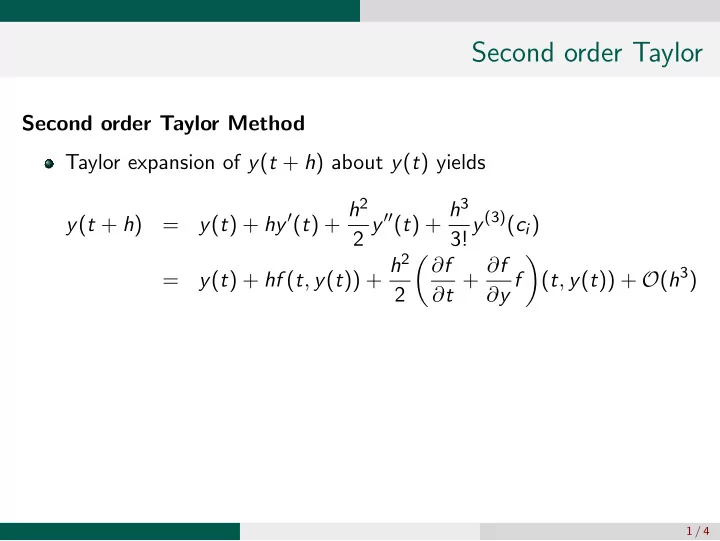
Second order Taylor Method Taylor expansion of y(t + h) about y(t) yields y(t + h) = y(t) + hy′(t) + h2 2 y′′(t) + h3 3! y(3)(ci) = y(t) + hf (t, y(t)) + h2 2 ∂f ∂t + ∂f ∂y f
- (t, y(t)) + O(h3)
1 / 4