Radiosity Radiosity Radiosity Radiosity Motivation: what is - - PDF document

SLIDE 1

1

Radiosity Radiosity

Radiosity Radiosity

• Motivation: what is missing in ray

Motivation: what is missing in ray-

• traced images?

traced images?

• Indirect illumination effects

Indirect illumination effects

• Color bleeding

Color bleeding

• Soft shadows

Soft shadows

• Radiosity

Radiosity is a physically is a physically-

• based illumination algorithm capable

based illumination algorithm capable

• f simulating the above phenomena in a scene made of ideal
• f simulating the above phenomena in a scene made of ideal

diffuse surfaces. diffuse surfaces.

• Books:

Books:

• Cohen and Wallace,

Cohen and Wallace, Radiosity Radiosity and Realistic Image Synthesis, and Realistic Image Synthesis, Academic Press Professional 1993. Academic Press Professional 1993.

• Sillion

Sillion and and Puech Puech, , Radiosity Radiosity and Global Illumination, Morgan and Global Illumination, Morgan-

• Kaufmann

Kaufmann, 1994. , 1994.

Indirect illumination effects Indirect illumination effects

Light source Diffuse Reflection Eye

Radiosity Radiosity in a Nutshell in a Nutshell

• Break surfaces into many small elements

Break surfaces into many small elements

• Formulate and solve a linear system of equations

Formulate and solve a linear system of equations that models the equilibrium of inter that models the equilibrium of inter-

• reflected

reflected light in a scene. light in a scene.

• The solution gives us the amount of light leaving

The solution gives us the amount of light leaving each point on each surface in the scene. each point on each surface in the scene.

• Once solution is computed, the shaded elements

Once solution is computed, the shaded elements can be quickly rendered from any viewpoint. can be quickly rendered from any viewpoint.

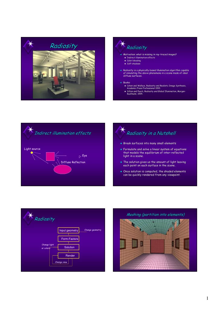
Radiosity Radiosity

Input geometry Form-Factors Solution Render

Change light

• r colors

Change view Change geometry

Meshing (partition into elements) Meshing (partition into elements)

SLIDE 2

2 Radiometric quantities Radiometric quantities

• Radiant energy [J]

Radiant energy [J]

• Radiant power (flux): radiant energy per second [W]

Radiant power (flux): radiant energy per second [W]

• Irradiance (flux density): incident radiant power per

Irradiance (flux density): incident radiant power per unit area [W/m unit area [W/m2

2]

]

• Radiosity

Radiosity (flux density): outgoing radiant power per (flux density): outgoing radiant power per unit area [W/m unit area [W/m2

2]

]

• Radiance (angular flux density): radiant power per

Radiance (angular flux density): radiant power per unit projected area per unit solid angle [W/(m unit projected area per unit solid angle [W/(m2

2 sr

sr)] )]

The The Radiosity Radiosity Equation Equation

• Assume that surfaces in the scene have been

Assume that surfaces in the scene have been discretized discretized into into n n small elements. small elements.

• Assume that each element emits/reflects light

Assume that each element emits/reflects light uniformly across its surface. uniformly across its surface.

• Define the

Define the radiosity radiosity B B as the total hemispherical as the total hemispherical flux density (W/m flux density (W/m2

2) leaving a surface.

) leaving a surface.

• Let

Let’ ’s write down an expression describing the s write down an expression describing the total flux (light power) leaving element total flux (light power) leaving element i i in the in the scene: scene: total flux = emitted flux + reflected flux total flux = emitted flux + reflected flux

The The Radiosity Radiosity Equation Equation

• Total flux leaving element i:

Total flux leaving element i:

• Total flux emitted by element i:

Total flux emitted by element i:

• Total reflected flux:

Total reflected flux:

• (reflectance of element i)*(the total incoming flux)

(reflectance of element i)*(the total incoming flux)

• total incoming flux = sum of contributions from all other

total incoming flux = sum of contributions from all other elements in the scene elements in the scene

• The full

The full radiosity radiosity equation is then: equation is then:

i iA

B

i iA

E

∑

j ji j j i

F A B ρ

∑

=

+ =

n j ji j j i i i i i

F A B A E A B

1

ρ

The Form Factor The Form Factor

• The form factor

The form factor F Fji

ji tells us how much of the flux

tells us how much of the flux leaving element j actually reaches element i. leaving element j actually reaches element i.

y x A x A y y x i ij

dA dA y x V y x A F

i j

∫ ∫

∈ ∈

− = ) , ( cos cos 1

2

π θ θ

Form Form-

• Factor Computation

Factor Computation Properties of Form Factors Properties of Form Factors

• Reciprocity:

Reciprocity:

• Additivity

Additivity: :

• Conservation of energy in a closed environment:

Conservation of energy in a closed environment:

ji j ij i

F A F A =

ik ij k j i

F F F + =

∪ ) (

1

1

=

∑

= n j ij

F

SLIDE 3

3 The The Radiosity Radiosity Equation Equation

• The

The radiosity radiosity equation equation

• Divide equation by A

Divide equation by Ai

i:

:

• Apply form

Apply form-

• factor reciprocity:

factor reciprocity:

• We can write this using matrix notation:

We can write this using matrix notation:

∑

=

+ =

n j ji j j i i i i i

F A B A E A B

1

ρ

∑

=

+ =

n j ji A A j i i i

F B E B

i j

1

ρ

∑

=

+ =

n j ij j i i i

F B E B

1

ρ ⎥ ⎥ ⎥ ⎦ ⎤ ⎢ ⎢ ⎢ ⎣ ⎡ ⎥ ⎥ ⎥ ⎦ ⎤ ⎢ ⎢ ⎢ ⎣ ⎡ + ⎥ ⎥ ⎥ ⎦ ⎤ ⎢ ⎢ ⎢ ⎣ ⎡ = ⎥ ⎥ ⎥ ⎦ ⎤ ⎢ ⎢ ⎢ ⎣ ⎡

n n n

B B E E B B M M M

1 1 1

Finally... Finally...

• A linear system of n equations in n unknowns:

A linear system of n equations in n unknowns: ⎥ ⎥ ⎥ ⎥ ⎦ ⎤ ⎢ ⎢ ⎢ ⎢ ⎣ ⎡ = ⎥ ⎥ ⎥ ⎥ ⎦ ⎤ ⎢ ⎢ ⎢ ⎢ ⎣ ⎡ ⎥ ⎥ ⎥ ⎥ ⎦ ⎤ ⎢ ⎢ ⎢ ⎢ ⎣ ⎡ − − − − − − −

n n nn n n n n

E E E B B B F F F F F F F M M L L M O M M L

2 1 2 1 1 22 2 21 2 1 1 12 1 11 1

1 1 1 ρ ρ ρ ρ ρ ρ ρ

The The Radiosity Radiosity Method Method

• Take as input a geometric model of the scene, with

Take as input a geometric model of the scene, with emission and reflection properties of each surface emission and reflection properties of each surface

• Step 1

Step 1 -

• Meshing

Meshing: : Discretize Discretize input surfaces into a input surfaces into a mesh of small elements mesh of small elements

• Step 2

Step 2 -

• Setup

Setup: Compute the form factors : Compute the form factors F Fij

ij

• Step 3

Step 3 -

• Solution

Solution: Solve the resulting linear : Solve the resulting linear system of equations system of equations

• Step 4

Step 4 -

• Display

Display: Render shaded elements from : Render shaded elements from any desired view point. any desired view point.

• These steps are often interleaved in practice.

These steps are often interleaved in practice.

Examples: Examples: Examples: Examples: Examples: Examples:

SLIDE 4

4 Solving the Equation Solving the Equation

• The naive approach

The naive approach -

• Gaussian

Gaussian elimination elimination

• Requires O(n

Requires O(n2

2) memory to store the matrix

) memory to store the matrix

• Requires O(n

Requires O(n3

3) time to solve the equation

) time to solve the equation

• A better approach

A better approach -

• iterative solution

iterative solution

• Jacobi

Jacobi iteration iteration

• Gauss

Gauss-

• Seidel iteration

Seidel iteration

• Southwell

Southwell relaxation (known as relaxation (known as Progressive Progressive Radiosity Radiosity) )

• Due to special properties of the

Due to special properties of the radiosity radiosity matrix, it is matrix, it is possible to prove that these iterative methods are possible to prove that these iterative methods are guaranteed to converge to the correct solution. guaranteed to converge to the correct solution.

Progressive Progressive Radiosity Radiosity

• While not converged:

While not converged:

• Select one element in the scene as the current light source

Select one element in the scene as the current light source

• “

“Shoot Shoot” ” radiosity radiosity from the light source to the rest of the scene from the light source to the rest of the scene

• The solution process mimics the physical process of light

The solution process mimics the physical process of light propagation in the scene. propagation in the scene.

• Must take care not to shoot the same light more than once

Must take care not to shoot the same light more than once (keep track of (keep track of “ “unshot radiosity unshot radiosity” ”) ) B[i] = Unshot[i] = E[i] B[i] = Unshot[i] = E[i] while (not converged) { while (not converged) { Choose i with largest Unshot[i]*A[i] Choose i with largest Unshot[i]*A[i] Shoot(i) Shoot(i) } }

Progressive Progressive Radiosity Radiosity

Shoot(i): Shoot(i): for j = 1..n { for j = 1..n { Compute the form factor FF[i,j] Compute the form factor FF[i,j] Delta[j] = Delta[j] = ρ ρ[j] FF[i,j] [j] FF[i,j] Unshot Unshot[i] A[i]/A[j] [i] A[i]/A[j] B[j] += Delta[j] B[j] += Delta[j] Unshot Unshot[j] += Delta[j] [j] += Delta[j] } } Unshot Unshot[i] = 0 [i] = 0 B[i] = Unshot[i] = E[i] B[i] = Unshot[i] = E[i] while (not converged) { while (not converged) { Choose i with largest Unshot[i]*A[i] Choose i with largest Unshot[i]*A[i] Shoot(i) Shoot(i) } }

Progressive Progressive Radiosity Radiosity

• In each iteration the algorithm computes n form factors on

In each iteration the algorithm computes n form factors on the fly, removing the O(n the fly, removing the O(n2

2) storage complexity.

) storage complexity.

• Choosing the

Choosing the “ “brightest brightest” ” shooter at each iteration makes shooter at each iteration makes the solution to converge rapidly during the first iterations. the solution to converge rapidly during the first iterations.

• It is possible to display the solution after each iteration,

It is possible to display the solution after each iteration, resulting in a progressive sequence of images. resulting in a progressive sequence of images.

• Typically, there is no need to run until complete convergence.

Typically, there is no need to run until complete convergence. The process can be stopped after relatively few iterations. The process can be stopped after relatively few iterations.

Progressive Radiosity Example: Progressive Radiosity Example: 0, 8, 16, 25, 50, 100 iterations 0, 8, 16, 25, 50, 100 iterations Progressive Radiosity + Ambient Progressive Radiosity + Ambient 0, 8, 16, 25, 50, 100 iterations 0, 8, 16, 25, 50, 100 iterations

SLIDE 5

5

Progressive Radiosity with Adaptive Progressive Radiosity with Adaptive Meshing (0,8,16,50,100) Meshing (0,8,16,50,100)

Form Form-

• Factor Computation

Factor Computation

• Analytic as well as approximate formulas exist for various

Analytic as well as approximate formulas exist for various configurations. configurations.

• A closed form expression for a form factor between two

A closed form expression for a form factor between two polygons ( polygons (Schroder Schroder 93): 93):

• extremely complicated formula

extremely complicated formula

• does not take into account occlusion

does not take into account occlusion

• A common approximation is to assume that the inner integral

A common approximation is to assume that the inner integral is constant for all locations x in element i: is constant for all locations x in element i:

∫ ∫ ∫

∈ ∈ ∈

≈ =

j i j

A y y y x y x A x A y y x i ij

dA y x V r dA dA y x V r A F ) , ( cos cos ) , ( cos cos 1

2 2

π θ θ π θ θ

Form Form-

• Factor Computation

Factor Computation Form Form-

• Factor Computation

Factor Computation

• The remaining integral is approximated as a finite sum:

The remaining integral is approximated as a finite sum:

• This approximation works well so long as the elements i and j

This approximation works well so long as the elements i and j are are well well-

• separated

separated from each other (the distance between from each other (the distance between them is large relative to their sizes) them is large relative to their sizes)

∑ ∫

Δ ≈ ≈

∈ y y x A y y y x ij

A y x V r dA y x V r F

j

) , ( cos cos ) , ( cos cos

2 2

π θ θ π θ θ

Nusselt Nusselt’ ’s s Method Method Hemicube Hemicube

SLIDE 6

6

SLIDE 7

7