
SLIDE 1
1 Radiosity
Don Greenberg Michael Cohen
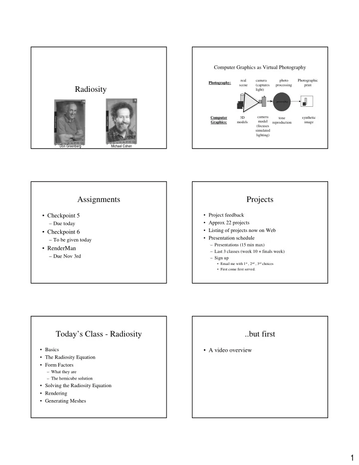
Computer Graphics as Virtual Photography
camera (captures light) synthetic image camera model (focuses simulated lighting)
processing
photo processing tone reproduction real scene 3D models Photography: Computer Graphics: Photographic print
Assignments
- Checkpoint 5
– Due today
- Checkpoint 6
– To be given today
- RenderMan
– Due Nov 3rd
Projects
- Project feedback
- Approx 22 projects
- Listing of projects now on Web
- Presentation schedule
– Presentations (15 min max) – Last 3 classes (week 10 + finals week) – Sign up
- Email me with 1st , 2nd , 3rd choices
- First come first served.
Today’s Class - Radiosity
- Basics
- The Radiosity Equation
- Form Factors
– What they are – The hemicube solution
- Solving the Radiosity Equation
- Rendering
- Generating Meshes
..but first
- A video overview