[PDF] - Radiosity Radiosity Cornell box with color bleeding [Goral et al PDF Document

SLIDE 1

Computer Graphics (Spring 2008) Computer Graphics (Spring 2008)

COMS 4160, Lecture 23: Radiosity

http://www.cs.columbia.edu/~cs4160

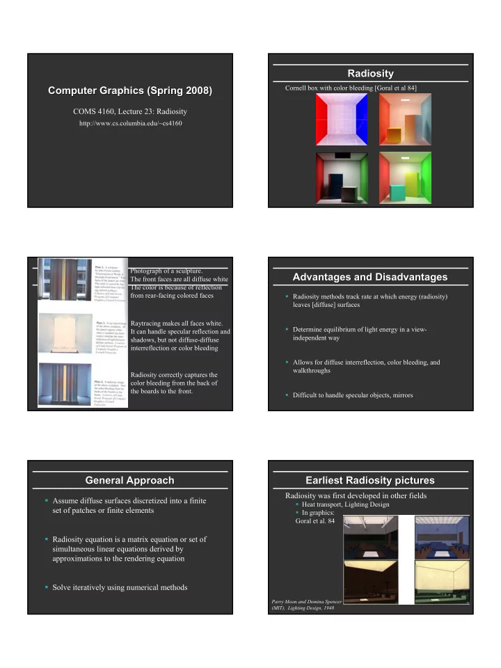
Radiosity Radiosity

Cornell box with color bleeding [Goral et al 84] Photograph of a sculpture. The front faces are all diffuse white The color is because of reflection from rear-facing colored faces Raytracing makes all faces white. It can handle specular reflection and shadows, but not diffuse-diffuse interreflection or color bleeding Radiosity correctly captures the color bleeding from the back of the boards to the front.

Advantages and Disadvantages Advantages and Disadvantages

Radiosity methods track rate at which energy (radiosity) leaves [diffuse] surfaces Determine equilibrium of light energy in a view- independent way Allows for diffuse interreflection, color bleeding, and walkthroughs Difficult to handle specular objects, mirrors

General Approach General Approach

Assume diffuse surfaces discretized into a finite set of patches or finite elements Radiosity equation is a matrix equation or set of simultaneous linear equations derived by approximations to the rendering equation Solve iteratively using numerical methods

Earliest Earliest Radiosity Radiosity pictures pictures

Radiosity was first developed in other fields

Heat transport, Lighting Design In graphics: Goral et al. 84

Parry Moon and Domina Spencer (MIT), Lighting Design, 1948

SLIDE 2

Outline Outline

Rendering equation review Radiosity equation Form factors Methods to compute form factors

High-level overview only. Best textual reference is probably Sections 16.3.1 and 16.3.2 in FvDFH. This will be handed out. If curious, read the rest of 16.3 and parts of Cohen and Wallace.

Rendering Equation

i

ω

r

ω

x

( , ) ( , , ) c ( , ) ( , )

s

e r i r r r i i r i

L x L x L x f x d ω ω ω ω θ ω ω

Ω

= + ′ −

∫

Reflected Light (Output Image) Emission Reflected Light BRDF Cosine of Incident angle i

dω

Surfaces (interreflection)

dA x′

UNKNOWN UNKNOWN KNOWN KNOWN KNOWN

i

x x ω ′− ∼

Change of Variables

Integral over angles sometimes insufficient. Write integral in terms of surface radiance only (change of variables) ( , ) ( , ) ( , ) ( , , ) cos

r r e r r i i r i i

L x L x L x d f x ω ω ω ω ω ω θ

Ω

′ = + −

∫

x x′

dA′

i

ω

i

ω −

i

θ

θ

i

dω

2

cos | |

i

dA d x x θ ω ′ = ′ −

Change of Variables

Integral over angles sometimes insufficient. Write integral in terms of surface radiance only (change of variables) ( , ) ( , ) ( , ) ( , , ) cos

r r e r r i i r i i

L x L x L x d f x ω ω ω ω ω ω θ

Ω

′ = + −

∫

2

cos | |

i

dA d x x θ ω ′ = ′ −

all visible 2 to

cos cos ( , ) ( , ) ( , ) ( , , ) | |

i

r

r e r r i i r x x

L x L x L x f x x d x A θ θ ω ω ω ω ω

′

′ = + − ′ − ′

∫

2

cos cos ( , ) ( , ) | |

i

G x x

G x x x x θ θ ′ ′ = = ′ −

Rendering Equation: Standard Form

Integral over angles sometimes insufficient. Write integral in terms of surface radiance only (change of variables) Domain integral awkward. Introduce binary visibility fn V ( , ) ( , ) ( , ) ( , , ) cos

r r e r r i i r i i

L x L x L x d f x ω ω ω ω ω ω θ

Ω

′ = + −

∫

2

cos | |

i

dA d x x θ ω ′ = ′ −

all visible 2 to

cos cos ( , ) ( , ) ( , ) ( , , ) | |

i

r

r e r r i i r x x

L x L x L x f x x d x A θ θ ω ω ω ω ω

′

′ = + − ′ − ′

∫

2

cos cos ( , ) ( , ) | |

i

G x x

G x x x x θ θ ′ ′ = = ′ −

all surfaces

( , ) ( , ) ( , ) ( , , ) ( , ) ( , )

r r e r r x i i r

L x L x L x f x G x dA x x V x ω ω ω ω ω

′

′ ′ ′ = + − ′

∫

Same as equation 2.52 Cohen Wallace. It swaps primed And unprimed, omits angular args of BRDF, - sign. Same as equation above 19.3 in Shirley, except he has no emission, slightly diff. notation

Radiosity Equation

all surfaces

( , ) ( , ) ( , ) ( , , ) ( , ) ( , )

r r e r r x i i r

L x L x L x f x G x dA x x V x ω ω ω ω ω

′

′ ′ ′ = + − ′

∫

Drop angular dependence (diffuse Lambertian surfaces) ( ) ( ) ( ) ( ) ( , ) ( , )

S r e r

L x L x f x L x G dA x x V x x ′ ′ ′ = + ′

∫

Change variables to radiosity (B) and albedo (ρ) ( , ) ( , ) ( ) ( ) ( ) ( )

S

G x x V x x B x E x x B x dA ρ π ′ ′ ′ = + ′

∫

Same as equation 2.54 in Cohen Wallace handout (read sec 2.6.3) Ignore factors of π which can be absorbed. Expresses conservation of light energy at all points in space

SLIDE 3

Outline Outline

Rendering equation review Radiosity equation Form factors Methods to compute form factors

Section 16.3.1,2 (eqs 16.63-65) in FvDFH

Discretization Discretization and Form Factors and Form Factors

( , ) ( , ) ( ) ( ) ( ) ( )

S

G x x V x x B x E x x B x dA ρ π ′ ′ ′ = + ′

∫

j i i i j j i j i

A B E B F A ρ

→

= + ∑

F is the form factor. It is dimensionless and is the fraction of energy leaving the entirety of patch j (multiply by area of j to get total energy) that arrives anywhere in the entirety of patch i (divide by area of i to get energy per unit area or radiosity).

Form Factors Form Factors

j

dA

i

θ

j

θ

i

dA

r

j

A

i

A ( , ) ( , )

i i j j j i i j

G x x V x x A F A F dAdA π

→ →

′ ′ = = ∫∫

2

cos cos ( , ) ( , ) | |

i

G x x

G x x x x θ θ ′ ′ = = ′ −

Matrix Equation Matrix Equation

j i i i j j i j i

A B E B F A ρ

→

= + ∑

( , ) ( , )

i i j j j i i j

G x x V x x A F A F dAdA π

→ →

′ ′ = = ∫∫

i i i j i j j

B E B F ρ

→

= + ∑

i i j i j i j

B B F E ρ

→

− =

∑

ij j i ij ij i i j j

M B E MB E M I F ρ

→

= = = −

∑

Outline Outline

Rendering equation review Radiosity equation Form factors Methods to compute form factors

Section 16.3.2 in FvDFH

Nusselt Nusselt’ ’s s Analog Analog

Analytically project into hemisphere above

point. Then project
nto hemisphere base

Form factor is ratio

f area on base to

area of entire base This computes differential point to patch form factor

Why does it work?

SLIDE 4

Hemicube Hemicube Hemicubes Hemicubes

Each small hemicube cell has a precomputed delta form factor: add up to get final value We can render the scene using normal Z-buffer scan conversion onto the faces of the hemicube!