
SLIDE 1
1
Foundations of Computer Graphics Foundations of Computer Graphics (Spring 2010) (Spring 2010)
CS 184, Lecture 21: Radiosity
http://inst.eecs.berkeley.edu/~cs184
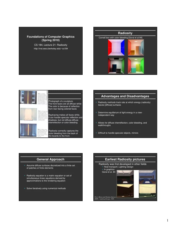
Radiosity Radiosity
Cornell box with color bleeding [Goral et al 84] Photograph of a sculpture. The front faces are all diffuse white The color is because of reflection from rear-facing colored faces Raytracing makes all faces white. It can handle specular reflection and shadows, but not diffuse-diffuse interreflection or color bleeding Radiosity correctly captures the color bleeding from the back of the boards to the front.
Advantages and Disadvantages Advantages and Disadvantages
- Radiosity methods track rate at which energy (radiosity)
leaves [diffuse] surfaces
- Determine equilibrium of light energy in a view-
independent way
- Allows for diffuse interreflection, color bleeding, and
walkthroughs
- Difficult to handle specular objects, mirrors
General Approach General Approach
- Assume diffuse surfaces discretized into a finite set
- f patches or finite elements
- Radiosity equation is a matrix equation or set of
simultaneous linear equations derived by approximations to the rendering equation
- Solve iteratively using numerical methods
Earliest Earliest Radiosity Radiosity pictures pictures
Radiosity was first developed in other fields
- Heat transport, Lighting Design
- In graphics:
Goral et al. 84
Parry Moon and Domina Spencer (MIT), Lighting Design, 1948