the rendering equation
play

The Rendering Equation Direct ( local ) illumination Light directly - PDF document

The Rendering Equation Direct ( local ) illumination Light directly from light sources No shadows Indirect ( global ) illumination 
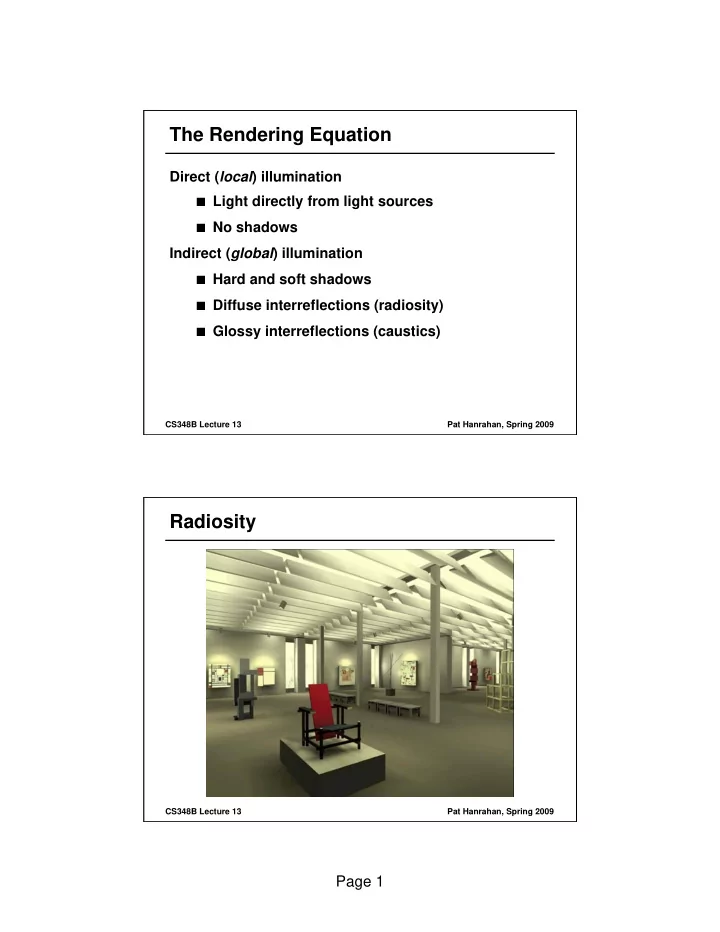
Hard and soft shadows Diffuse interreflections (radiosity) Glossy


  1. The Rendering Equation Direct ( local ) illumination � � Light directly from light sources � � No shadows Indirect ( global ) illumination � � Hard and soft shadows � � Diffuse interreflections (radiosity) � � Glossy interreflections (caustics) CS348B Lecture 13 Pat Hanrahan, Spring 2009 Radiosity CS348B Lecture 13 Pat Hanrahan, Spring 2009 Page 1

  2. Lighting Effects Hard Shadows Soft Shadows Caustics Indirect Illumination CS348B Lecture 13 Pat Hanrahan, Spring 2009 Challenge To evaluate the reflection equation the incoming radiance must be known To evaluate the incoming radiance the reflected radiance must be known CS348B Lecture 13 Pat Hanrahan, Spring 2009 Page 2

  3. To The Rendering Equation Questions 1. How is light measured? 2. How is the spatial distribution of light energy described? 3. How is reflection from a surface characterized? 4. What are the conditions for equilibrium flow of light in an environment? CS348B Lecture 13 Pat Hanrahan, Spring 2009 The Grand Scheme Light and Radiometry Energy Balance Surface Volume Rendering Equation Rendering Equation Radiosity Equation CS348B Lecture 13 Pat Hanrahan, Spring 2009 Page 3

  4. Energy Balance Balance Equation Accountability [ outgoing ] - [ incoming ] = [ emitted ] - [ absorbed ] � � Macro level The total light energy put into the system must equal the energy leaving the system (usually, via heat). � � Micro level The energy flowing into a small region of phase space must equal the energy flowing out. CS348B Lecture 13 Pat Hanrahan, Spring 2009 Page 4

  5. Surface Balance Equation [ outgoing ] = [ emitted ] + [ reflected ] CS348B Lecture 13 Pat Hanrahan, Spring 2009 Direction Conventions BRDF Surface vs. Field Radiance CS348B Lecture 13 Pat Hanrahan, Spring 2009 Page 5

  6. Surface Balance Equation [ outgoing ] = [ emitted ] + [ reflected ] + [ transmitted ] BTDF CS348B Lecture 13 Pat Hanrahan, Spring 2009 Two-Point Geometry Ray Tracing CS348B Lecture 13 Pat Hanrahan, Spring 2009 Page 6

  7. Coupling Equations Invariance of radiance CS348B Lecture 13 Pat Hanrahan, Spring 2009 The Rendering Equation Directional form Transport operator i.e. ray tracing Integrate over hemisphere of directions CS348B Lecture 13 Pat Hanrahan, Spring 2009 Page 7

  8. The Rendering Equation Surface form Geometry term Integrate over all surfaces Visibility term CS348B Lecture 13 Pat Hanrahan, Spring 2009 The Radiosity Equation Assume diffuse reflection 1. 2. CS348B Lecture 13 Pat Hanrahan, Spring 2009 Page 8

  9. Integral Equations Integral Equations Integral equations of the 1 st kind Integral equations of the 2 nd kind CS348B Lecture 13 Pat Hanrahan, Spring 2009 Page 9

  10. Linear Operators Linear operators act on functions like matrices act on vectors They are linear in that Types of linear operators CS348B Lecture 13 Pat Hanrahan, Spring 2009 Solving the Rendering Equation Rendering Equation Solution CS348B Lecture 13 Pat Hanrahan, Spring 2009 Page 10

  11. Formal Solution Neumann series Verify CS348B Lecture 13 Pat Hanrahan, Spring 2009 Successive Approximations Successive approximations Converged CS348B Lecture 13 Pat Hanrahan, Spring 2009 Page 11

  12. Successive Approximation CS348B Lecture 13 Pat Hanrahan, Spring 2009 Paths Page 12

  13. Light Path CS348B Lecture 13 Pat Hanrahan, Spring 2009 Light Path CS348B Lecture 13 Pat Hanrahan, Spring 2009 Page 13

  14. Light Paths CS348B Lecture 13 Pat Hanrahan, Spring 2009 Light Transport Integrate over all paths of all lengths Question: � � How to sample space of paths? CS348B Lecture 13 Pat Hanrahan, Spring 2009 Page 14

  15. Classic Ray Tracing From Heckbert Forward (from eye): E S* (D|G) L CS348B Lecture 13 Pat Hanrahan, Spring 2009 Photon Paths Radiosity Caustics From Heckbert CS348B Lecture 13 Pat Hanrahan, Spring 2009 Page 15

  16. How to Solve It? Finite element methods � � Classic radiosity � � Mesh surfaces � � Piecewise constant basis functions � � Solve matrix equation � � Not practical for rendering equation Monte Carlo methods � � Path tracing (distributed ray tracing) � � Bidirectional ray tracing � � Photon mapping CS348B Lecture 13 Pat Hanrahan, Spring 2009 Page 16

Download Presentation
Download Policy: The content available on the website is offered to you 'AS IS' for your personal information and use only. It cannot be commercialized, licensed, or distributed on other websites without prior consent from the author. To download a presentation, simply click this link. If you encounter any difficulties during the download process, it's possible that the publisher has removed the file from their server.

Recommend


More recommend