Image-Based Rendering and Modeling l Image-based rendering (IBR): - PDF document

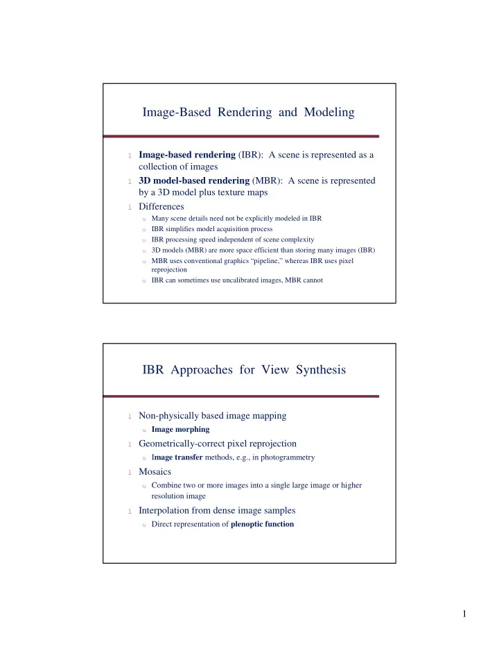
Image-Based Rendering and Modeling l Image-based rendering (IBR): A scene is represented as a collection of images l 3D model-based rendering (MBR): A scene is represented by a 3D model plus texture maps l Differences u Many scene details need not be explicitly modeled in IBR u IBR simplifies model acquisition process u IBR processing speed independent of scene complexity u 3D models (MBR) are more space efficient than storing many images (IBR) u MBR uses conventional graphics “pipeline,” whereas IBR uses pixel reprojection u IBR can sometimes use uncalibrated images, MBR cannot IBR Approaches for View Synthesis l Non-physically based image mapping u Image morphing l Geometrically-correct pixel reprojection u I mage transfer methods, e.g., in photogrammetry l Mosaics u Combine two or more images into a single large image or higher resolution image l Interpolation from dense image samples u Direct representation of plenoptic function 1

Image Metamorphosis (Morphing) l Goal : Synthesize a sequence of images that smoothly and realistically transforms objects in source image A into objects in destination image B l Method 1: 3D Volume Morphing u Create 3D model of each object u Transform one 3D object into another u Render synthesized 3D object u Hard/expensive to accurately model real 3D objects u Expensive to accurately render surfaces such as skin, feathers, fur 2

Image Morphing l Method 2: Image Cross-Dissolving u Pixel-by-pixel color interpolation u Each pixel p at time t ∈ [0, 1] is computed by combining a fraction of each pixel’s color at the same coordinates in images A and B: p = (1 - t ) p A + t p B p A p p B t 1-t u Easy, but looks artificial, non-physical Image Morphing l Method 3: Mesh-based image morphing u G. Wolberg, Digital Image Warping , 1990 u Warp between corresponding grid points in source and destination images u Interpolate between grid points, e.g., linearly using three closest grid points u Fast, but hard to control so as to avoid unwanted distortions 3

Image Warping l Goal: Rearrange pixels in an image. I.e., map pixels in source image A to new coordinates in destination image B l Applications u Geometric Correction (e.g., due to lens pincushion or barrel distortion) u Texture mapping u View synthesis u Mosaics l Aka geometric transformation , geometric correction , image distortion l Some simple mappings: 2D translation, rotation, scale, affine, projective Image Warping image plane in front image plane below black area where no pixel maps to 4

Homographies l Perspective projection of a plane u Lots of names for this: u homography , texture-map, colineation, planar projective map u Modeled as a 2D warp using homogeneous coordinates       sx' * * * x       = sy' * * * y              s   * * *    1 p ′ ′ ′ ′ H p To apply a homography H • Compute p ′ ′ ′ ′ = Hp (regular matrix multiply) • Convert p ′ ′ ′ ′ from homogeneous to image coordinates – divide by s (third) coordinate Examples of 2D Transformations Original Rigid Projective Affine 5

Mapping Techniques l Define transformation as either u Forward : x = X (u, v), y = Y (u, v) u Backward : u = U (x, y), v = V (x, y) Source Destination Image A Image B v y u x Mapping Techniques Forward, point-based l u Apply forward mapping X , Y at point (u,v) to obtain real-valued point (x,y) u Assign (u,v)’s gray level to pixel closest to (x,y) B A u Problem: “ measles ,” i.e., “ holes ” (pixel in destination image that is not assigned a gray level) and “ folds ” (pixel in destination image is assigned multiple gray levels) u Example: Rotation, since preserving length cannot preserve number of pixels 6

Mapping Techniques Forward, square-pixel based l u Consider pixel at (u,v) as a unit square in source image. Map square to a quadrilateral in destination image u Assign (u,v)’s gray level to pixels that the quadrilateral overlaps u Integrate source pixels’ contributions to each output pixel. Destination pixel’s gray level is weighted sum of intersecting source pixels’ gray levels, where weight proportional to coverage of destination pixel u Avoids holes, but not folds, and requires intersection test Mapping Techniques Backward, point-based l u For each destination pixel at coordinates (x,y), apply backward mapping, U , V , to determine real-valued source coordinates (u,v) u Interpolate gray level at (u,v) from neighboring pixels, and copy gray level to (x,y) u Interpolation may cause artifacts such as aliasing, blockiness, and false contours u Avoids holes and folds problems u Method of choice 7

Backward Mapping l For x = xmin to xmax for y = ymin to ymax u = U (x, y) v = V (x, y) B[x, y] = A[u, v] l But (u, v) may not be at a pixel in A l (u, v) may be out of A’s domain l If U and/or V are discontinuous, A may not be connected! l Digital transformations in general don’t commute Pixel Interpolation l Nearest-neighbor (0-order) interpolation u g(x, y) = gray level at nearest pixel (i.e., round (x, y) to nearest integers) u May introduce artifacts if image contains fine detail l Bilinear (1st-order) interpolation u Given the 4 nearest neighbors, g(0, 0), g(0, 1), g(1, 0), g(1, 1), of a ≤ ≤ desired point g(x, y), compute gray level at g(x, y): 0 x , y 1 , u Interpolate linearly between g(0,0) and g(1,0) to obtain g(x,0) u Interpolate linearly between g(0,1) and g(1,1) to obtain g(x,1) u Interpolate linearly between g(x,0) and g(x,1) to obtain g(x,y) u Combining all three interpolation steps into one we get: u g(x,y) = (1-x)(1-y) g(0,0) + (1-x)y g(0,1) + x(1-y) g(1,0) + xy g(1,1) l Bicubic spline interpolation 8

Bilinear Interpolation l A simple method for resampling images Example of Backward Mapping l Goal : Define a transformation that performs a scale change, which expands size of image by 2, i.e., U (x) = x/2 l A = 0 … 0 2 2 2 0 … 0 l 0-order interpolation, I.e., u =  x/2  B = 0 … 0 2 2 2 2 2 2 0 … 0 l Bilinear interpolation, I.e., u = x/2 and average 2 nearest pixels if u is not at a pixel B = 0 … 0 1 2 2 2 2 2 1 0 … 0 9

Image Morphing l Method 4: Feature-based image morphing u T. Beier and S. Neely, Proc. SIGGRAPH ‘92 u Distort color and shape ⇒ image warping + cross-dissolving u Warping transformation partially defined by user interactively specifying corresponding pairs of line segment features in the source and destination images; only a sparse set is required (but carefully chosen) u Compute dense pixel correspondences, defining continuous mapping function, based on weighted combination of displacement vectors of a pixel from all of the line segments u Interpolate pixel positions and colors (2D linear interpolation) Beier and Neely Algorithm l Given : 2 images, A and B, and their corresponding sets of line segments, L A and L B , respectively l Foreach intermediate frame time t ∈ [0, 1] do u Linearly interpolate the position of each line u L t [i] = Interpolate(L A [i], L B [i], t) u Warp image A to destination shape u WA = Warp(A, L A , L t ) u Warp image B to destination shape u WB = Warp(B, L B , L t ) u Cross-dissolve by fraction t u MorphImage = CrossDissolve(WA, WB, t) 10

Example: Translation l Consider images where there is one line segment pair, and it is translated from image A to image B: A M .5 B l First, linearly interpolate position of line segment in M l Second, for each pixel (x, y) in M, find corresponding pixels in A (x-a, y) and B (x+a, y), and average them Feature-based Warping l Goal : Define a continuous function that warps a source image to a destination image from a sparse set of corresponding, oriented, line segment features - each pixel’s position defined relative to these line segments l Warping with one line pair: foreach pixel p B in destination image B do find dimensionless coordinates (u,v) relative to oriented line segment q B r B find p A in source image A using (u,v) relative to q A r A p B copy color at p A to p B r A r B Destination v Image B Source v u p A Image A u q B q A 11

Feature-based Warping (cont.) l Warping with multiple line pairs u Use a weighted combination of the points defined by the same mapping q’ 1 q 1 q 2 X X v 2 X ′ 1 q’ 2 v 1 v 1 u 2 X ′ ′ ′ ′ v 2 u 1 p 2 u 1 X ′ 2 u 2 p’ 2 p 1 p’ 1 Destination Image Source Image X ′ ′ ′ = weighted average of D 1 and D 2 , where D i = X ′ i - X , ′ and weight = (length(p i q i ) c / (a + |v i |)) b , for constants a, b, c 12

Geometrically-Correct Pixel Reprojection l What geometric information is needed to generate virtual camera views? u Dense pixel correspondences between two input views u Known geometric relationship between the two cameras u Epipolar geometry View Interpolation from Range Maps l Chen and Williams, Proc. SIGGRAPH ‘93 (seminal paper on image-based rendering) l Given : Static 3D scene with Lambertian surfaces, and two images of that scene, each with known camera pose and range map l Algorithm : 1. Recover dense pixel correspondence using known camera calibration and range maps 2. Compute forward mapping, X F , Y F , and backward mapping, X B , Y B . Each “morph map” defines an offset vector for each pixel 13