IBR Approaches for View Synthesis Image-Based Rendering and - - PowerPoint PPT Presentation

1 Image-Based Rendering and Modeling

l Image-based rendering (IBR): A scene is represented as a

collection of images

l 3D model-based rendering (MBR): A scene is represented

by a 3D model plus texture maps

l Differences

u Many scene details need not be explicitly modeled in IBR u IBR simplifies model acquisition process u IBR processing speed independent of scene complexity u 3D models (MBR) are more space efficient than storing many images (IBR) u MBR uses conventional graphics “pipeline,” whereas IBR uses pixel

reprojection

u IBR can sometimes use uncalibrated images, MBR cannot

IBR Approaches for View Synthesis

l Non-physically based image mapping

u Image morphing

l Geometrically-correct pixel reprojection

u Image transfer methods, e.g., in photogrammetry

l Mosaics

u Combine two or more images into a single large image or higher

resolution image

l Interpolation from dense image samples

u Direct representation of plenoptic function

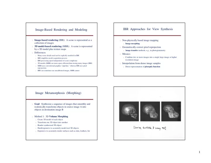
Image Metamorphosis (Morphing)

l Goal: Synthesize a sequence of images that smoothly and

realistically transforms objects in source image A into

• bjects in destination image B

l Method 1: 3D Volume Morphing

u Create 3D model of each object u Transform one 3D object into another u Render synthesized 3D object u Hard/expensive to accurately model real 3D objects u Expensive to accurately render surfaces such as skin, feathers, fur

2 Image Morphing

l Method 2: Image Cross-Dissolving

u Pixel-by-pixel color interpolation u Each pixel p at time t ∈ [0, 1] is computed by combining a fraction

• f each pixel’s color at the same coordinates in images A and B:

p = (1 - t) pA + t pB

u Easy, but looks artificial, non-physical

pA pB p t 1-t

Image Morphing

l Method 3: Mesh-based image morphing

u G. Wolberg, Digital Image Warping, 1990 u Warp between corresponding grid points in source and destination

images

u Interpolate between grid points, e.g., linearly using three closest grid

points

u Fast, but hard to control so as to avoid unwanted distortions

Image Warping

l Goal: Rearrange pixels in an image. I.e., map pixels in

source image A to new coordinates in destination image B

l Applications

u Geometric Correction (e.g., due to lens pincushion or barrel

distortion)

u Texture mapping u View synthesis u Mosaics

l Aka geometric transformation, geometric correction,

image distortion

l Some simple mappings: 2D translation, rotation, scale,

affine, projective

Image Warping

image plane in front image plane below

black area where no pixel maps to

3 Homographies

l Perspective projection of a plane

u Lots of names for this:

u homography, texture-map, colineation, planar projective map

u Modeled as a 2D warp using homogeneous coordinates

sx' * * * x sy' * * * y s * * * 1             =                  

H p p′ ′ ′ ′ To apply a homography H

• Compute p′

′ ′ ′ = Hp (regular matrix multiply)

• Convert p′

′ ′ ′ from homogeneous to image coordinates – divide by s (third) coordinate

Examples of 2D Transformations

Original Rigid Affine Projective

Mapping Techniques

Destination Image B x y

l Define transformation as either

u Forward: x = X(u, v), y = Y(u, v) u Backward: u = U(x, y), v = V(x, y)

Source Image A u v

Mapping Techniques

l

Forward, point-based

u Apply forward mapping X, Y at point (u,v) to obtain real-valued point (x,y) u Assign (u,v)’s gray level to pixel closest to (x,y) u Problem: “measles,” i.e., “holes” (pixel in destination image that is not

assigned a gray level) and “folds” (pixel in destination image is assigned multiple gray levels)

u Example: Rotation, since preserving length cannot preserve number of

pixels

A B

4 Mapping Techniques

l

Forward, square-pixel based

u Consider pixel at (u,v) as a unit square in source image. Map square to a

quadrilateral in destination image

u Assign (u,v)’s gray level to pixels that the quadrilateral overlaps u Integrate source pixels’ contributions to each output pixel. Destination

pixel’s gray level is weighted sum of intersecting source pixels’ gray levels, where weight proportional to coverage of destination pixel

u Avoids holes, but not folds, and requires intersection test

Mapping Techniques

l

Backward, point-based

u For each destination pixel at coordinates (x,y), apply backward mapping,

U, V, to determine real-valued source coordinates (u,v)

u Interpolate gray level at (u,v) from neighboring pixels, and copy gray

level to (x,y)

u Interpolation may cause artifacts such as aliasing, blockiness, and false

contours

u Avoids holes and folds problems u Method of choice

Backward Mapping

l For x = xmin to xmax

for y = ymin to ymax u = U(x, y) v = V(x, y) B[x, y] = A[u, v]

l But (u, v) may not be at a pixel in A l (u, v) may be out of A’s domain l If U and/or V are discontinuous, A may not be connected! l Digital transformations in general don’t commute

Pixel Interpolation

l Nearest-neighbor (0-order) interpolation

u g(x, y) = gray level at nearest pixel (i.e., round (x, y) to nearest

integers)

u May introduce artifacts if image contains fine detail

l Bilinear (1st-order) interpolation

u Given the 4 nearest neighbors, g(0, 0), g(0, 1), g(1, 0), g(1, 1), of a

desired point g(x, y), compute gray level at g(x, y):

u Interpolate linearly between g(0,0) and g(1,0) to obtain g(x,0) u Interpolate linearly between g(0,1) and g(1,1) to obtain g(x,1) u Interpolate linearly between g(x,0) and g(x,1) to obtain g(x,y)

u Combining all three interpolation steps into one we get:

u g(x,y) = (1-x)(1-y) g(0,0) + (1-x)y g(0,1) + x(1-y) g(1,0) + xy g(1,1)

l Bicubic spline interpolation

, 1 , ≤ ≤ y x

5 Bilinear Interpolation

l A simple method for resampling images

Example of Backward Mapping

l Goal: Define a transformation that performs a scale change,

which expands size of image by 2, i.e., U(x) = x/2

l A = 0 … 0 2 2 2 0 … 0 l 0-order interpolation, I.e., u = x/2

B = 0 … 0 2 2 2 2 2 2 0 … 0

l Bilinear interpolation, I.e., u = x/2 and average 2 nearest

pixels if u is not at a pixel

B = 0 … 0 1 2 2 2 2 2 1 0 … 0

Image Morphing

l Method 4: Feature-based image morphing

u T. Beier and S. Neely, Proc. SIGGRAPH ‘92 u Distort color and shape

⇒ image warping + cross-dissolving

u Warping transformation partially defined by user interactively

specifying corresponding pairs of line segment features in the source and destination images; only a sparse set is required (but carefully chosen)

u Compute dense pixel correspondences, defining continuous

mapping function, based on weighted combination of displacement vectors of a pixel from all of the line segments

u Interpolate pixel positions and colors (2D linear interpolation)

Beier and Neely Algorithm

l Given: 2 images, A and B, and their corresponding sets of

line segments, LA and LB, respectively

l Foreach intermediate frame time t ∈ [0, 1] do

u Linearly interpolate the position of each line

u L t[i] = Interpolate(LA[i], LB[i], t)

u Warp image A to destination shape

u WA = Warp(A, LA, Lt)

u Warp image B to destination shape

u WB = Warp(B, LB, Lt)

u Cross-dissolve by fraction t

u MorphImage = CrossDissolve(WA, WB, t)

6 Example: Translation

l Consider images where there is one line segment pair, and

it is translated from image A to image B:

l First, linearly interpolate position of line segment in M l Second, for each pixel (x, y) in M, find corresponding

pixels in A (x-a, y) and B (x+a, y), and average them A B M.5

Feature-based Warping

l Goal: Define a continuous function that warps a source

image to a destination image from a sparse set of corresponding, oriented, line segment features - each pixel’s position defined relative to these line segments

l Warping with one line pair:

foreach pixel pB in destination image B do

find dimensionless coordinates (u,v) relative to oriented line segment qBrB find pA in source image A using (u,v) relative to qArA copy color at pA to pB

qA rA pA

u v

qB rB pB

u v Source Image A Destination Image B

Feature-based Warping (cont.)

l Warping with multiple line pairs

u Use a weighted combination of the points defined by the same

mapping

p1 q1 p2 q2 u1 u2 v1 v2

X

p’1 q’1 u1 v1

X

q’2 p’2 u2 v2 Destination Image Source Image

X′ ′ ′ ′ X′ ′ ′ ′ = weighted average of D1 and D2, where Di = X′i - X, and weight = (length(piq i)c / (a + |vi|))b , for constants a, b, c

X′2 X′1

7 Geometrically-Correct Pixel Reprojection

l What geometric information is needed to generate virtual

camera views?

u Dense pixel correspondences between two input

views

u Known geometric relationship between the two

cameras

u Epipolar geometry

View Interpolation from Range Maps

l Chen and Williams, Proc. SIGGRAPH ‘93 (seminal paper

• n image-based rendering)

l Given: Static 3D scene with Lambertian surfaces, and two

images of that scene, each with known camera pose and range map

l Algorithm:

• 1. Recover dense pixel correspondence using known

camera calibration and range maps

• 2. Compute forward mapping, XF, YF, and backward

mapping, XB, YB. Each “morph map” defines an offset vector for each pixel

View Interpolation (cont.)

• 3. Compute interpolated “morph map” by linearly

interpolating forward and backward offset vectors, given intermediate frame, t,

• 4. Apply forward mapping from A given interpolated

morph map (approximating perspective transformation for new view)

• 5. Use a z-buffer (and A’s range map) to keep only closest

pixel (so, handles folds)

• 6. For each pixel in interpolated image that has no color,

interpolate color from all adjacent colored pixels 1 ≤ ≤ t

View Morphing

l Seitz and Dyer, Proc. SIGGRAPH ‘95 l Given: Two views of an unknown rigid scene, with no

camera information known, compute new views from a virtual camera at viewpoints in-between two input views

8

Photograph Photograph Photograph Photograph Morphed View Morphed View Virtual Camera Virtual Camera

When is View Synthesis Feasible?

l Given two images, I0 and I1, with optical centers C0 and

C1, if the monotonicity constraint holds for C0 and C1, then there is sufficient information to completely predict the appearance of the scene from all in-between viewpoints along line segment C0C1

l Monotonicity Constraint: All visible scene points appear

in the same order along conjugate epipolar line in I0 and I1

l Any number of distinct scenes could produce I0 and I1, but

each one produces the same in-between images

9

• 1. Prewarp

align views

• 1. Prewarp

align views

• 2. Morph

move camera

• 1. Prewarp

align views

• 2. Morph

move camera

• 3. Postwarp

point camera

10 Features of View Morphing

l Provides

u A mobile virtual camera u Better image morphs

l Requires no prior knowledge

u No 3D shape information u No camera information u No training on other images

Application: Photo Correction

l Image Postprocessing

u Alter image perspective in the lab

l Image Databases

u Normalize images for better indexing u Simplify face recognition tasks

Corrected Photographs Corrected Photographs Original Photographs Original Photographs

11 Another Example Application: Better Image Transitions

u Avoid bending and shearing distortions u Shapes do not need to be aligned

Image Morph Image Morph View Morph View Morph

Mosaics

l Goal: Given a static scene and a set of images (or video) of

it, combine the images into a single “panoramic image” or “panoramic mosaic”

l Motivation: Image-based modeling of 3D scenes benefits

visualization, navigation, exploration, VR walkthroughs, video compression, video stabilization, super-resolution

l Example: Apple’s Quicktime VR (Chen, SIGGRAPH ‘95)

Image Mosaics

l

+ + … + =

l Goal

u Stitch together several images into a seamless composite

12 Mosaicing Method

l Registration: Given n input images, I1, …, In, compute an

image-to-image transformation that will map each image I2, …, In into the coordinate frame of reference image, I1

l Warp: Warp each image Ii, i=2, …, n, using transform l Interpolate: Resample warped image l Composite: Blend images together to create single output

image based on the reference image’s coordinate frame

When can Two Images be Aligned?

l

Problems

u In general, warping function depends on the depth of the

corresponding scene point since image projection defined by x′ = fx/z, y′ = fy/z

u Different views means, in general, that parts that are visible in one

image may be occluded in the other

l

Special cases where the above problems can’t occur

u Panoramic mosaic: Camera rotates (i.e., pans) about its optical

center, arbitrary 3D scene

u No motion parallax as camera rotates, so depth unimportant u 2D projective transformation relates any 2 images (⇒ 8

unknowns)

u Planar mosaic: Arbitrary camera views of a planar scene

u 2D projective transformation relates any 2 images

13

How to Determine Alignment Assuming a Planar Projective Transformation between Cameras?

l Method 1: Find 4 point correspondences, and then solve

for 8 unknowns

u Requires reliable detection of four corresponding features, at sub-

pixel location accuracy

l Method 2: Use image-based (intensity) correlation to

determine best matching transformation

u No correspondences needed u Statistically optimal (gives maximum likelihood estimate) u Useful for local image registration

Example: 2D Rigid Warp Mosaics

l Assume: Planar scene, camera motion restricted to plane

parallel to scene, optical axis perpendicular to scene, intensity constancy assumption, local displacement

l 3 unknowns: 2D translation (a, b) and 2D rotation (θ) l Relation between two images, I and I′, given by:

y I y x b x I x y a y x I y x I I y x b y x y a x I y x I b y x a y x I y x I ∂ ∂ − + + ∂ ∂ − − + ≈ ′ ′ ′ − + + − − + ≈ ′ ′ ′ + + + − = ′ ′ ′ / ) 2 / ( / ) 2 / ( ) , ( ) , ( : expansion series Taylor its

• f

m first ter to Expanding ) 2 / , 2 / ( ) , ( : series Taylor in terms first two to cos and sin Expanding ) cos sin , sin cos ( ) , (

2 2 2 2

θ θ θ θ θ θ θ θ θ θ θ θ θ θ

Example: 2D Rigid Warp Mosaics

l Solve for a, b, θ that minimizes SSD error: l Assuming small displacement, use gradient descent to

minimize E, ∇E = (∂E/∂a, ∂E/∂b, ∂E/∂θ)

l Iteratively update total motion estimate, (a, b, θ), while

warping I′ towards I until E < threshold

∑∑ ∑∑

− ∂ ∂ − + + ∂ ∂ + − + = − ′ =

x y

y x I y I y x b x I x y a y x I I I E

2 2 2 2

)) , ( / ) 2 / ( / ) 2 / ( ) , ( ( ) ( θ θ θ θ

2D Rigid Warp Algorithm

l Because the displacement between images may not be

small enough to solve directly for the motion parameters, use an iterative algorithm instead:

• 1. a(0) = 0; b(0) = 0; θ(0) = 0; m = (0, 0, 0); t = 1
• 2. Solve for a(t), b(t), θ(t) from the 3 equations
• 3. Update the total motion estimate:

m(t+1) = m(t) + (a(t), b(t), θ(t))

• 4. Warp I′ toward I: I′ = warp(I′, a(t), b(t), θ(t) )
• 5. If (a(t) < ε1 and b(t) < ε2 and θ(t) < ε3 )

then halt else t = t + 1; goto step 2

14 Dealing with Noisy Data: RANSAC

l How to find the best fitting data to a global model when

the data are noisy – especially because of the presence of

• utliers, i.e., missing features and extraneous features?

l RANSAC (Random Sample Consensus) Method u Iteratively select a small subset of data and fit model to

that data

u Then check all of data to see how many fit the model

RANSAC Algorithm for Robust Estimation

bestcnt := 0 until there is a good fit or k iterations do randomly choose a sample of n points from the dataset compute the best fitting model parameters to the selected subset of the n data points cnt := 0 foreach remaining data point do if the distance from the current point to the model is < T then cnt++ if cnt ≥ D then there is a good fit, so re-compute the best fitting model parameters using all of the good points, and halt else if cnt > bestcnt then bestcnt := cnt

Other Robust Parameter Estimation Methods

l How to deal with outliers, i.e., occasional large-scale

measurement errors?

l M-Estimators

u Generalization of

u MLE (Maximum Likelihood Estimation) u LMedS (Least Median of Squares)

u

is the set of model parameters, ρ is a “robust loss function” whose shape is parameterized by σ, and ri (xi,

) is the residual error of the model

with the ith data element

∑

∈X x i i

i

x r ) ); , ( ( min arg σ θ ρ

θ

15 Least Median of Squares (LMedS)

l Defined as l Up to ½ of data points can be arbitrarily far from the optimum

estimate without changing the result

l Median is not differentiable, so how to search for optimum? u Use randomization:

u Randomly select a subset of the data u Compute model,

, from the selected subset

u Each candidate model,

, is tested by computing r2 using the remaining data points and selecting the median of these values

) , ( median min arg

2

θ

θ i X x

x r

i∈

Global Image Registration

l When images are not sufficiently close, must do global

registration

l Method 1: Coarse-to-fine matching using Gaussian

Pyramid

• 1. Compute Gaussian pyramids
• 2. level = N // Set initial processing level to coarse level
• 3. Solve for motion parameters at level level
• 4. If level = 0 then halt
• 5. Interpolate motion parameters at level level - 1
• 6. level = level - 1
• 7. Goto step 3

Global Image Registration

l Method 2: Coarse-to-fine matching using Laplacian

Pyramid

u Use Laplacian pyramids, LA and LB u for l = N to 0 step -1 do

Use motion estimate from previous iteration to warp level l in LA for do compute cross-correlation at level l: smooth using Gaussian pyramid to level S: foreach (x,y) interpolate 3 x 3 correlation surface centered at (x,y) at level S to find peak, corresponding to best local motion estimate find best-fit global motion model to flow field ) , ( ) , ( ) , (

,

j y i x LB y x LA y x CC

l l j i

+ + = ) , ( * ) , ( ) , (

, ,

y x w y x CC y x C

j i j i

= 1 , 1 ≤ ≤ − j i

Planar Mosaics and Panoramic Mosaics

l Motion model is 2D projective transformation, so 8

parameters

l Assuming small displacement, minimize SSD error l Apply (nonlinear) minimization algorithm to solve

16 Panoramic Mosaics

l Large field of view ⇒ can’t map all images onto a plane l Instead, map onto cylinder, sphere, or cube l Example: With a cylinder, first warp all images from

rectilinear to cylindrical coordinates, then mosaic them

l “Undistort” (perspective correct) image from this

representation prior to viewing

Cylindrical panoramas

l Steps

u Reproject each image onto a cylinder u Blend u Output the resulting mosaic

f = 180 (pixels)

Cylindrical reprojection

l Map image to cylindrical coordinates

u need to know the camera focal length

Image 384x300 f = 380 f = 280

Cylindrical image stitching

l

What if you don’t know the camera rotation?

u Solve for the camera rotations

u Note that a rotation of the camera is a translation of the cylinder! u Use Lucas-Kanade to solve for translations of cylindrically-warped images

17 Full-view Panorama

+ + + + + + + +

Other types of mosaics

l

Can mosaic onto any surface if you know the geometry

u See NASA’s Visible Earth project for some stunning earth mosaics

u

http://earthobservatory.nasa.gov/Newsroom/BlueMarble/

Path Images

x y t

Pushbroom image

http://grail.cs.washington.edu/projects/stereo/

18 Cyclograph

http://grail.cs.washington.edu/projects/stereo/

Multi-Perspective Image

Rademacher and Bishop,1998

Some Blending Methods

l Average intensity of overlapping pixels l Median intensity of overlapping pixels l Newest (i.e., most recent frame) pixel’s intensity l Burt’s pyramid blending method l Bilinear blending

u Weighted average with pixels near center of each image contributing

more

u Let wt be a 1D triangle (hat) function of size equal to width of

image, with value 0 at edges and value 1 at midpoint. Then use 2D weighting function:

) ( ) ( ) , (

i t i t i i

y w x w y x w ′ ′ = ′ ′

Image Blending

19 Feathering

1 1

+ =

Encoding transparency I(x,y) = (αR, αG, αB, α) Iblend = Ileft + Iright

(J. Blinn, CGA, 1994) for details

Effect of window size

1

left right

1

Effect of window size

1 1

Good window size

1

l

“Optimal” window: smooth but not ghosted

u Doesn’t always work...

20 Mosaicing Arbitrary Scenes

l For general scenes and arbitrary viewpoints, we must

recover depth

l Method 1: Depth map given ala Chen and Williams l Method 2: Segment image into piecewise-planar patches

and use 2D projective method for each patch

l Method 3: Recover dense 3D depth map using either

stereo reconstruction (assuming known motion between cameras) or structure from motion (assuming no camera motion is known)

Learning-based View Synthesis from 1 View

l Vetter and Poggio, IEEE Trans. PAMI, 1997 l Given: A set of views of several training objects, and a

single view of a new object

l Single view of new object considered to be approximated

by a linear combination of views of the training objects, all at the same pose as the new object

l Learn set of weights that specify best match between given

view of new object and same view of the training objects

l Use learned weights with other views of training objects to

synthesize novel view of new object

Approach: Example-based Modeling of Faces 2D Image 3D Face Models 2D Image 3D Face Models

= w1* + w2* + w3* + w4* +.

Cylindrical Coordinates

red(h,φ) green(h,φ) blue(h,φ) red(h,φ) green(h,φ) blue(h,φ) φ h radius(h,φ) radius(h,φ) h φ

21

=

a1 * + a2 * + a3 * + a4 * + . . . b1 * +b2 * +b3* +b4* + . . .

Vector Space of 3D Faces

lA Morphable Model can generate new faces

Modeling in Face Space

Caricature Original Original Average Average

Modeling the Appearance of Faces

A face is represented as a point in face space

lWhich directions code for specific attributes?

3D Shape from Images

Face Analyzer

3D Head 3D Head Input Image Input Image

22 Matching a Morphable 3D Face Model

= R

Optimization problem! Optimization problem! Optimization problem!

a1 * + a2 * + a3 * + a4 * + . . . b1 * + b2 * + b3 * + b4 * + . . .

23 3D Modeling from a photograph Criminisi et al., ICCV 99

l Complete approach

u Load in an image u Click on lines parallel to X axis

u repeat for Y, Z axes

u Compute vanishing points u Specify 3D and 2D positions of 4 points on reference plane u Compute homography H u Specify a reference height u Compute 3D positions of several points u Create a 3D model from these points u Extract texture maps u Output a VRML model

C

Measurements within reference plane

l

Solve for homography H relating reference plane to image plane

u H maps reference plane (X,Y) coords to image plane (x,y) coords u Fully determined from 4 known points on ground plane

u Option A: physically measure 4 points on ground u Option B: find a square, guess the dimensions

u Given (x, y), can find (X,Y) by H-1

reference plane

[ ]

T

Y X 1

[ ]

T

y x 1 image plane

24

C

Measuring height without a ruler

ground plane

l Compute Y from image measurements

u Need more than vanishing points to do this

Y

The cross ratio

l

A Projective Invariant

u Something that does not change under projective transformations

(including perspective projection)

P1 P2 P3 P4

1 4 2 3 2 4 1 3

P P P P P P P P − − − −

The cross-ratio of 4 collinear points

l

Can permute the point ordering

u 4! = 24 different orders (but only 6 distinct values) l

This is the fundamental invariant of projective geometry             = 1

i i i i

Z Y X P

3 4 2 1 2 4 3 1

P P P P P P P P − − − −

vZ r t b

t v b r r v b t − − − −

Z Z

image cross ratio

Measuring height

B (bottom of object) T (top of object) R (reference point) ground plane H C

T B R R B T − ∞ − − ∞ −

scene cross ratio

∞ ∞ ∞ ∞

            = 1 Z Y X P           = 1 y x p scene points represented as image points as

R H = R H =

R

l For a given scene, describe

ALL rays through

u ALL pixels, of u ALL cameras, at u ALL wavelengths, u ALL time

F(x,y,z, φ φ φ φ,θ θ θ θ, λ λ λ λ, t)

“eyeballs everywhere” function (5D x 2D)

Plenoptic Function (Adelson and Bergen 1991)

… … … … … … … … … … … … … … … … … … … … … …

25 Plenoptic Array: ‘The Matrix Effect’

l Brute force! Simple arc, line, or ring array of cameras l Synchronized shutter – Dayton Taylor’s TimeTrack l Warp/blend between images to change viewpoint on ‘time-

frozen’ scene:

How Much Light is Really in a Scene?

l

Light transported throughout scene along rays

u Anchor

u Any point in 3D space u 3 coordinates

u Direction

u Any 3D unit vector u 2 angles

u Total of 5 dimensions l

Radiance remains constant along ray as long as in empty space

u Removes one dimension u Total of 4 dimensions

L1 L2 dA1 dA2 dω1 dω2

radiance constant here

Light Field and Lumigraph

l Light Field

u Levoy & Hanrahan, Siggraph 1996

l Lumigraph

u Gortler et al., Siggraph 1996

l Consider (u,v) the image plane and (s,t)

the viewpoint plane

l Photographs taken from a bunch of

different viewpoints

l Reconstructed photographs of scene are

2D slices of 4D light field

l View scene through a window l All visible light from scene must have passed through

window

l Window light is 4D

u 2 coordinates where ray intersects window pane u 2 angles for ray direction

l Use a double-paned window

u 2 coordinates (u,v) where ray intersects first pane u 2 coordinates (s,t) where ray intersects second pane

s t u v

Representing All of the Light in a Scene

26 Object Based

l Can be made a cube around object

Images from uv Plane Making Light Field/Lumigraph

l Rendered from synthetic model l Made from real world u With gantry u Handheld

27 Gantry

l Lazy Susan

u Manually rotated

l XY Positioner l Lights turn with lazy susan l Correctness by construction

Handheld Camera

l Blue screen on stage u Walls moveable, can turn

Ray Tracing and Light Fields

l Rendering into a light field

u Cast rays between all pairs of points in panes u Store resulting radiance at (u,v,s,t)

l Rendering from a light field

u Cast rays through pixels into light field u Compute two ray-plane intersections to find (u,v,s,t) u Interpolate u,v and s,t to find radiance between samples u Plot radiance in pixel

Results

28 Results

l Light Field