
SLIDE 1
1
Radiosity
A good book on radiosity: Radiosity Global Illumination, F. X. Sillion, C. Puech, Morgan Kaufmann publishers, INC., 1994.
Introduction
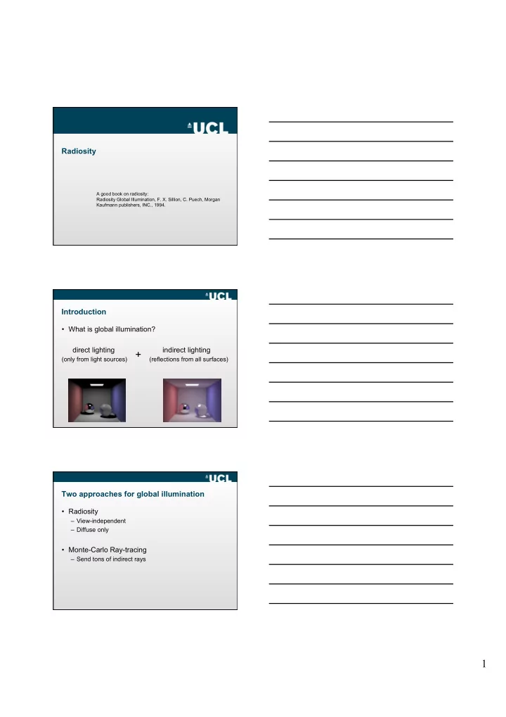
- What is global illumination?
direct lighting indirect lighting
(only from light sources) (reflections from all surfaces)
+
Two approaches for global illumination
- Radiosity
– View-independent – Diffuse only
- Monte-Carlo Ray-tracing
– Send tons of indirect rays