Query Processing University of Wisconsin Madison Specializing in - - PowerPoint PPT Presentation

1

Query Processing

Jon Frankel, Noi Jencharat, Ened Ketri, Anurag Maskey, Andy See, Larissa Smelkov 3/25/03

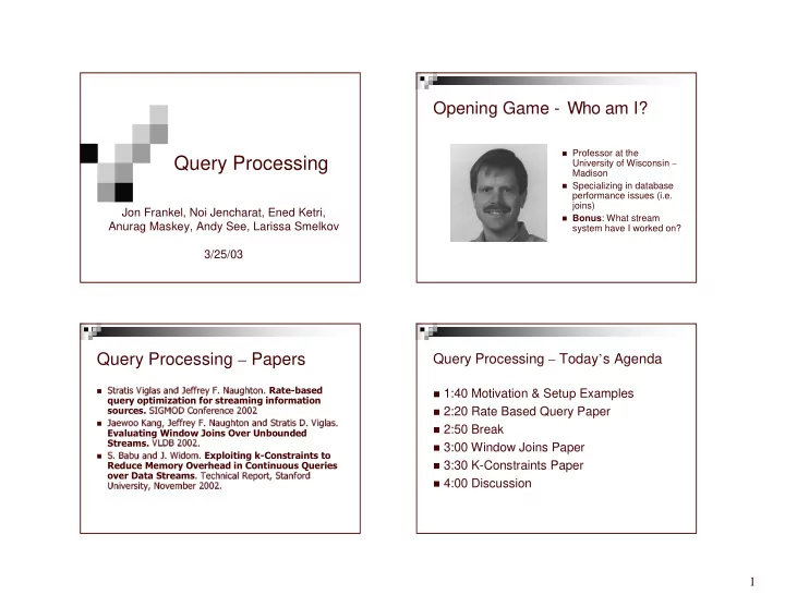
Opening Game - Who am I?

• Professor at the

University of Wisconsin – Madison

• Specializing in database

performance issues (i.e. joins)

• Bonus: What stream

system have I worked on?

Query Processing – Papers

• ✁

• ✁✗

• ☞

• ✞✩

• ✁

!"# $%#& '

Query Processing – Today’s Agenda

1:40 Motivation & Setup Examples

2:20 Rate Based Query Paper

2:50 Break

3:00 Window Joins Paper

3:30 K-Constraints Paper

4:00 Discussion

2

127 Flashback

• Optimizer - cost based
• Select * from students

where major = ‘cosi’ and birthday = ‘0325’

SQL Query Parser/ Translator Plan Generator Rewriter Evaluator Final Data Optimizer

Stream Challenges

• Final Answer?
• Block Reads?
• Cardinality?

Stream Challenges

• Final Answer?
• Block Reads?
• Cardinality?

Rate Based Cost Estimating

• Load Shedding
• Ad Hoc Queries
• Persistent Queries

Rate Based Analysis

MFC – 10/day; JDF 3/day

9 8 7 6

1 -> 0

5

1 3 -> 1 2 -> 1

4

3 3 -> 1 2 10 -> 5 12

3

1 3 -> 1 9 -> 4 9

2

3 -> 1 6 -> 3 6

1 Left JDF Left MFC New Day

3

Rate Based Analysis

MFC – 10/day; JDF 3/day

3 -> 1

9

3 3 -> 1

8

6 3 -> 1

7

9 3 -> 1

6

12 3 -> 1 1 -> 0

5

15 3 -> 1 1 3 -> 1 2 -> 1

4

18 3 -> 1 3 3 -> 1 2 10 -> 5 12

3

9 3 -> 1 1 3 -> 1 9 -> 4 9

2

3 3 -> 1 3 -> 1 6 -> 3 6

1 Left MFC Left JDF Left JDF Left MFC New Day

Rate Based Analysis

MFC – 10/day; JDF 3/day

9 -> 4 3 -> 1

9

3 3 -> 1

8

6 3 -> 1

7

9 3 -> 1

6

12 3 -> 1 1 -> 0

5

15 3 -> 1 1 3 -> 1 2 -> 1

4

18 3 -> 1 3 3 -> 1 2 10 -> 5 12

3

9 3 -> 1 1 3 -> 1 9 -> 4 9

2

3 3 -> 1 3 -> 1 6 -> 3 6

1 Left MFC Left JDF Left JDF Left MFC New Day

Cost Optimization

• Speed??

Coming Up….

• Different ways to

measure rates

• SPJ applicability

127 Flashback – Joins

Predicate Pushdown

Select * from students as s, courses as c where s.major = ‘cosi’

and c.dept = ‘cosi’ and s.sid = c.sid

4

Stream Challenges II

• Blocking Query Operators
• (option: pipelined join)
• Lost/Delayed/Unordered

Data

• And yet, benefits are

huge…

A C1 B D1 D2 E C2 A B1 C D F E B2

Stream Challenges II

• Blocking Query Operators
• (option: pipelined join)
• Lost/Delayed/Unordered

Data

• And yet, benefits are

huge…

A C1 B D1 D2 E C2 A B1 C D F E B2

Stock Market – Econ 2A

Stock prices are based on ?

S&P Federated Dept Stores Home Depot Papa John’s

Data is Out there!

(http://biz.yahoo.com/cc/)

Thu Mar 20 Times are U.S. Eastern 8:30 am CYCL Centennial Communications Earnings (Q3 2003) 8:30 am DV DeVry Inc. Acquires Ross University 8:30 am ENTG Entegris, Inc. Earnings (Q2 2003) 8:30 am PLXS Plexus Announcement 9:00 am HOLL Hollywood Media Corp. Fourth Quarter and Year-End 2002 9:00 am LEH Lehman Brothers Holdings First Quarter 2003 Earnings 10:00 am CSCO Cisco Systems Announces Agreement to Acquire The Linksys Group, Inc. 10:00 am FNLY Finlay Enterprises, Inc. Earnings (Q4 2002) 10:00 am GIII G-III Apparel Group Earnings (Q4 2003) 10:00 am GLYN Galyan's Trading Company, Inc. Fourth Quarter 2002 10:00 am MWD Morgan Stanley Earnings (Q1 2003) 10:00 am TRMS Trimeris, Inc. Earnings (Q4 2002) 10:30 am GPN Global Payments Inc. Earnings (Q3 2003) 11:00 am GDT Biosensor`s Agreement/Drug Eluting Stent Update 11:00 am CRAI Charles River Associates Earnings (Q1 2003) 11:00 am CHKR Checkers Drive-In Restaurants Earnings (Q4 2002) 11:00 am CPWM Cost Plus Earnings (Q4 2002) 11:00 am JCREW J. Crew Group, Inc. Earnings (Q4 2003)

5

Stocks & Stream Systems

• 2. HD 0.30
• 1. HD 0.27
• 1. IBM 80.00
• 1. INTC 15.00
• 1. HD 22.00
• 2. IBM 80.50
• 2. INTC 22.25
• 5. HD 22.75
• 9. HD 23.00

EPS (actual) EPS (est)

Tickers

Query: Short-term Downward Momentum: Find all NASDAQ stocks between $20 and $200 that have moved down more than 2% in the last 20 minutes and there has been significant buying pressure (70% or more of the volume has traded toward the ask price) in the last 2 minutes.

Or by: Earnings, News, Industry

Aurora Example

1, T1, C 2, T1, C 1, T2, B 2, T2, C 3, T1, A 3, T2, C 1, S1, A 1, S2, A 2, S1, A 1, S3, B 2, S3, B 3, S1, A 3, S3, B 2, S2, C 3, S2, B

Problem? Tanks

(time, ID, pos)

Soldiers

(time, ID, pos) A S1, S2 C T1 B T2, S3 A S1 C T1, T2, S2 B S3 A T1, S1 C T2, S2 B S3

Join Challenges – Window Options

• Aurora Option (by

individual tuple)

• Stream Option (slide)

Tuple vs Timestamp A C1 B D1 D2 E C2 A B1 C D F E B2

Order!

6

Join Challenges – Window Options

• Aurora Option (by

individual tuple)

• Stream Option (slide)

Tuple vs Timestamp A C1 B D1 D2 E C2 A B1 C D F E B2

Order!

Join Challenges – Window Options

• Aurora Option (by

individual tuple)

• Stream Option (slide)

Tuple vs Timestamp A C1 B D1 D2 E C2 A B1 C D F E B2

Order!

Join Challenges – Window Options

• Aurora Option (by

individual tuple)

• Stream Option (slide)

Tuple vs Timestamp A C1 B D1 D2 E C2 A B1 C D F E B2

Order!

Accuracy – How to window? Coming Up….

• Joining algorithms
• Lots of cool graphs

7

Motivations

Traditional Optimizers requires cardinality

• f the input….

In streams, cardinality is not known and inputs come at different rate…

RATE-BASED optimization

What is Rate?

Number of records per a unit of time.

Output Rate = # output transmitted time needed for transmission Output Rate = #papers processing time needed

Output Rate Estimation

For Projections

For Selections

For Joins

Output Rate for Projections

case 1: Mitch

Time to read papers is shorter than time between getting the papers

paper 1 paper 2 paper 3 1 hour 1/2 hour 1 hour

So the output rate = the input rate

paper 1 paper 2 paper 3 time

8

Output Rate for Projections

case 2: Jon

Time to read papers is longer than time between getting the papers

paper 1 paper 2 paper 3 1 hour 1.5 hour 1.5 hour

So the output rate = 1/(time to do projection)

time paper 1 paper 2

Output Rate for Projections

In general, time to do projection is low.

So Output Rate = Input Rate ro ri

Output Rate for Selections

Selectivity (f) = percentage of papers that will be selected

Output Rate for Selection

case 1: Mitch takes 1/2 hour to read 1 paper, with selectivity = 0.5

paper 1 paper 2 paper 3 1 hour 1/2 hour 2 hours

• utput rate = 1/2 paper/hour

So the output rate = f * the input rate

paper 1 time

9

Output Rate for Selection

case 2: John takes 1.5 hour to read 1 paper, with selectivity = 0.5

paper 1 paper 2 paper 3 1 hour 1.5 hour 3 hours

• utput rate = 1/3 paper/hour (= 1/2 * 1/1.5)

So the output rate = f * (1/time to select)

time

Output Rate for Selections

In general, time to perform selection is less than interval between inputs.

So Output Rate = Selectivity * Input Rate ro f * ri

Output Rate for Joins

What are the papers by same author Mitch and Jon gives the same grading to?

rM = No. of papers Mitch reads per hour

rJ = No. of papers Jon reads per hour

f = Selectivity of join

CM= Time to handle reviews from Mitch

CJ = Time to handle reviews from Jon

Recall

Output Rate = # output transmitted time needed for transmission

Total #’s of papers in output Total time to do the Join

10

Output Tuples

time interval = t:

We have: rM*t paper reviews from Mitch rJ*t paper reviews from Jon f*rM*rJ*t2 tuples that can be in the output.

after 1 hour

rM rJ f * rM * rJ Number of output tuples: f * rM * rJ

Mitch Jon Output

after 2 hours

rM rJ f * rM * rJ Number of output tuples:

f * rM * rJ

rM rJ + f*rM*2rJ + f*2rM*rJ

• f*rM*rJ

???

Mitch Jon Output

after 2 hours

rM rJ f * rM * rJ Number of output tuples:

f * rM * rJ + 3 * f * rM * rJ

rM rJ 3* f * rM * rJ

Mitch Jon Output

11

after 3 hours

rM rJ f * rM * rJ Number of output tuples:

f * rM * rJ + 3 * f * rM * rJ

rM rJ + f*rM*3rJ + f*3rM*rJ - f*rM*rJ 3* f * rM * rJ rM rJ ???

Mitch Jon Output

after 3 hours

rM rJ f * rM * rJ Number of output tuples:

f * rM * rJ + 3 * f * rM * rJ + 5* f * rM * rJ

rM rJ 3* f * rM * rJ rM rJ 5* f * rM * rJ

Mitch Jon Output

after time t

There will be (2t-1) f* rM * rJ new tuples in the output.

Total number of outputs at time t:

((2t-1) f* rM * rJ) dt

= t2 * f* rM * rJ – t* f* rM * rJ = f* rM * rJ * t *(t-1)

Time to Process Join

at time t Total time = rM*t * CM + rJ*t * CJ

= t( rM*CM + rJ* CJ)

rJ *t * CJ CJ rJ*t Jon rM*t * CM CM rM*t Mitch Processing Time Time Inputs

12

Output Rate for Joins

# output transmitted time needed for transmission = f* rM * rJ * t *(t-1) = f* rM * rJ *(t-1) t( rM*CM

+ rJ* CJ) ( rM*CM + rJ* CJ)

f* rM * rJ * t rM*CM

+ rJ* CJ

Optimizing Queries

# outputs =

Optimize for a specific time point

which plan will produce the most results by to?

Optimize for output production size

which plan is the first one to reach N results?

• p

dt t r ) (

Local Rate Maximization

Mitch Jon Students bottom-up rate maximization first, maximize

• utput rate here

then, maximize rate for this join

Local Time Minimization

Mitch Jon Students top-down time minimization n tuples in result first, minimize time to produce n tuples finally, minimize time to get the desired tuples

13

Experiment I the plans

A B C ( A B ) C ( A C ) B A B C (5K,20ms) (10K,2ms) (20K,10ms) A B A C A C B (5K,20ms) (10K,2ms) (20K,10ms) A C A B

Experiment I performance until last tuple

(5K,20ms)-(10K,2ms)-(20K,10ms) (5K,20ms)-(20K,10ms)-(10K,2ms) 50 100 150 200 250 300 50 100 150 200 250 20000 40000 60000 80000 100000

estimated measured

A B C A C B

Time (seconds) Output size number of tuples)

Experiment I

performance for the first few thousand tuples

20 40 60 80 100 5 10 15 20 25 30 35 40 1000 2000 3000 4000 5000 6000

estimated measured

A B C A C B

(5K,20ms)-(10K,2ms)-(20K,10ms) (5K,20ms)-(20K,10ms)-(10K,2ms)

Time (seconds) Output size number of tuples)

Complex Plans

D E D D D D D

D

E E

D D E E E

A (5K, 20ms) B (10K, 10ms) C (20K, 15ms) D (50k, 5ms) E (100K, 2ms)

C C C C C C A A A A A A A A B B B B B B B B B

(2) Fast Leaves

B A

(1) Left Deep (3) Evenly Spread

14

Experiment Result

Left Deep Fast Leaves Evenly Spread

600000 500000 400000 300000 200000 100000 0 200 400 600 800 1000 0 500 1000 1500

Ouput size (# tuples) Time (s) Estimated Measured

Comparison to Traditional Model

D D E

D

C C A A A B B B

(2) Fast Leaves

D D E

D E

C C A A A B B

(3) Evenly Spread

8.8 * 102 5 * 103 Evenly Spread 9.7 * 102 2 * 103 Fast Leaves 1.3 * 103 104 Left Deep Rate-Based Est. Traditional Est. Plan

E A (5K, 20ms) 100ms B (10K, 10ms) 100ms C (20K, 15ms) 300ms D (50k, 5ms) 250ms E (100K, 2ms) 200ms B

Evaluating Window Joins

• ver Unbounded Streams

Jaewoo Kang Jeffrey F. Naughton Stratis D. Viglas

University of Wisconsin- Madison Computer Sciences Department

Moving Window Join

15

Types of Join

Nested loops join

Hash join

Nested Loops Join Nested Loops Join Hash Join

Hash A Hash B

16

Open Questions

How to measure the efficiency of a moving

window join?

Can the join of streams with different rates

be more efficient?

How to deal with fast input streams when

system cannot manage them?

How to share limited memory between the

two windows for the two inputs?

Cost of Moving Window Joins (unit

• time
• b

asis model) Idea!

Streaming join algorithms can be asymmetric Hash – Nested Loops join Nested Loops – Hash join … or symmetric Nested Loops – Nested Loops join Hash – Hash join

Cost of Join

Nested loops join

Hash join

17

Comparison of Joins

NHJ HHJ NNJ HNJ

Full Joins Full Joins: different selectivity 1

• w

a y Join: System/Model cost

18

Overhead Costs

Ch/Cn

Ratio of overhead cost of Hash Join to Nested

Loop join

Model: ratio = 1.3

|B|

Number of hash buckets in window B,

assumed same as number of unique keys in window B

Variable that can be changed in the model

Crossover Points

Output rates

CPU time

19

Insufficient Resources for handling the Stream Input Rates

Problem

Very Expensive Predicates Input rate > Join operator service rate

Solution

Drop tuples from input

Resource Allocation Strategies Limited Memory

Variable Time Window Allocate Memory depending on Stream

Rate

Memory Allocation Strategies

20

Memory Allocation Strategies Memory Allocation Implications

Give all memory (biggest window size) to

slowest input stream

Fast stream probes slow stream, skips

insertion/invalidation

Full Join reduces to One Way Join on the

direction of slow fast

Choose Join Algorithm after memory

allocation

Conclusions

A Full Join can be seen as two separate

independent Single Joins

Exploit asymmetrical stream input rates

NLJ/HJ algorithms Combination

HNJ/NHJ best candidate

Resource allocation

Devote most resources to slowest stream

K-Constraints

Exploiting k-Constraints to Reduce Memory Overhead in Continuous Queries over Data Streams

Shivnath Babu and Jennifer Widom, Stanford University

21

Introduction

Already saw:

Use Rate information to optimize.

Now we’ll see

Use properties of streamed data. In order to reduce memory usage.

Outline

Constraints for streams K-constraints Synopsis Algorithm using k-constraints

Constraints

Properties that data streams satisfy. Examples:

Many-one join constraints between two streams. Referential-integrity constraints for streams

Between two streams in many-one join “One” side arrives before “Many” side

Clustered-arrival constraints on an attribute

Duplicate values arrive together

Ordered-arrival constraints on an attribute

Values are clustered and ordered.

Constraints (visual)

Referential

Integrity

Clustered Arrival Ordered Arrival

A B A B C B D

tuples Many-to-One

E C E C X A B A B C

tuples tuples

22

Constraints ?

How practical are these constraints for

streams?

Tuples may come out of order.

Clustered? Ordered?

Data rate may vary.

Referential Integrity?

K

• C
• nstraints

Idea: allow some disorder. K-Constraints are:

Constraints that are almost met. K is the adherence parameter

Lower K means streams comes closer to the

constraint.

Like “slack” in Aurora

Set amount of disorder can be tolerated by system.

Examples:

Referential Integrity

Many-one join from S1 to S2. S2 tuple will arrive before joining S1 tuple,

• r within K tuples on S2.

S1.A S2.A

A A A A B E G X B

K = 4

D Join on S1.A=S2.A

Clustered

• a

rrival

On attribute S.A: At most k tuples with different S.A values

arrive between tuples with the same value for S.A.

S.A

A A A B B

K=3

23

Ordered

• a

rrival

On stream attribute S.A: Tuples that arrive at least k+1 tuples after

tuple s have a value greater than or equal to s.

2 1 2 3 3

K=3

4

s S.A

The Idea

Joins over streams take infinite memory. Idea is to use k-constraints to reduce

memory usage

Slower increase in memory usage. Constant memory usage in some cases.

K-constraints can decide which tuples to

keep around.

Terminology

Synopsis: stream history Each Synopsis for a stream involved with a

query:

Has 3 components of seen tuples:

Yes: may contribute to a result tuple No: cannot contribute to a result tuple Unknown: cannot be put in Yes or No.

Join Graph: directed graph with arcs from

“Many” (parent) to the “One” (child) of many-one join.

Synopsis example

Query: Students that have GPA < 3.0 in Kalman when fire alarm is on.

Unknown No Yes Fire GPA Student

Stream Student gets tuple:

OUTPUT: Fire (location, time) GPA (stID, gpa) Student (stID, location, time) (id1234, Kalman, 12:00)

Stream Fire gets tuple:

(id1234, 2.9) (Edison, 12:00) (id1234, Kalman, 12:05) (Kalman, 12:05) (id1234, 2.9, Kalman, 12:05)

24

Synopsis

Why not just keep those tuples that are in

the Yes or Unknown synopsis?

Might cause tuples in other streams to be

kept in Unknown rather than being discarded.

Synopsis example 2

Soldiers with heartrate = 0 where more than 2 missiles were seen.

Unknown No Yes Missiles(Sector) Where(soldID,Sector) Heart(soldID, Rate)

Stream Heart (SoldierID,Rate) gets tuple:

OUTPUT

Stream Missile(Sector) gets tuple:

Missile (Sector, Number) Where (ID,Sector) Heart (ID,Rate) (s2,Sec5) (Sec3, 1) (s2,0,Sec5) (s1,1) (s2,0) (s3,Sec3) (s3,0) (Sec5, 4)

Referential Integrity

UNK NO YES Join heart rates greater than 35 with soldiers in sector 3 on id and time. Constraints:

• location gets

transmitted first

• always arrives

within 2 tuples of heart rate. sec2 s3 time loc id 1 sec2 s2 1 39 s1 time rate id 1 28 s1 2 sec3 s1 UNK NO YES many-one s1,2,sec3 s3,0,sec2 s1,1,39 s3,1,38 s3,1,sec3 s1,1,28 1 sec3 s3 s2,1,sec2 1 38 s3 Since more than 2 tuples have come on left, this can be moved to No. The No synopsis on left is never needed!!! Neither is No on the right. Many One OUTPUT: (s3,1,sec3,38) loc = sec3 rate > 35

Referential Integrity

If Referential Integrity with parameter K

holds on many-one join S1 to S2

Eliminate S2’s No component Keep S1’s Unknown component for only k

tuples on S2.

Location HeartRate

25

Ordered-Arrival Constraints (OA(k))

Two algorithms:

On child stream (“one” in many-one join)

OAC(k)

On parent stream (“many” in many-one join)

OAP(k)

Ordered Arrival (on “one”)

UNK NO YES Soldiers in sector 3 while a soldier had heart rate of

• 0. (Join on time.

Assume one location tuple per time.)

Constraint:

• Location comes

in ordered, with at most 1 tuples out

• f order.

1 sec2 s4 time loc id 2 sec2 s5 1 s2 time rate id 4 s1 4 sec3 s7 UNK NO YES many-one s7,4,sec3 s4, 1,sec2 s2,1,0 s3,0,38 s1,4,0 s5,2,sec2 38 s3 Since minimum on left will now be 2, we can move this to No!!! The No synopsis on left is never needed!!! Many One OUTPUT: (s7,s1, 2,sec3,0) rate =0 loc = sec3

Ordered Arrival (on “many”)

UNK NO YES Soldiers in sector 3 while a soldier had heart rate of

• 0. (Join on time.

Assume one location tuple per time.)

Constraint:

• HeartRate

comes in ordered, with at most 1 tuples out of

• rder.

sec3 s4 time loc id 5 sec2 s5 1 s2 time rate id 2 s1 2 sec3 s7 UNK NO YES many-one s7,2,sec3 s4, 0,sec3 s2,1,0 s3,2,38 s1,2,0 s5,5,sec2 2 38 s3 Since k+1 tuples with time > 0 have come

• n right, we can

discard this!! The No synopsis on left is never needed!!! Many One OUTPUT: (s7,s1, 2,sec3,0) rate =0 loc = sec3

OAC(k)

Similar to Referential Integrity Eliminate No synopsis without filling parent

Unknown synopsis:

Maintain the minimum value L that will be

seen on stream S.

Tuples in parent Stream less than L that

do not match S’s Unknown or Yes, must have no matching tuple in S – no need to put into Unknown.

26

OAP(k)

Idea:

Given a child stream’s tuple s, If no future parent tuples can join with s, Then, Don’t store s.

If Ordered Arrival constraint on parent

stream’s attribute A OAP(k)

Can drop child’s tuples after k tuples with

larger A values.

Clustered Arrival (CA(k))

Idea:

Similar to Ordered arrival on parent stream.

If parent streams have CA(k) on attribute

A:

After a joining tuple in parent, store s for only k

more parent tuples.

RIDS(k) Results Larger k means tuples are kept in Unknown synopsis longer, using more memory. CA(k) Results Smaller K means store fewer tuples in child streams Yes synopsis

27

OAP(k) Results Smaller K means store less in child Yes synopsis OAC(k) Results Smaller K means tuples are kept in parent stream synopsis less time. CA(k) and OAC(k) Combining CA(k) and OAC(k) does better than either alone, especially at high values for K.

CA(k) vs. combined CA(k) and RIDS(k) Note that at low K for RIDS(k), CA(k) does better. Some tuples are kept around longer than in pure CA(k).

28

Summary

Accuracy Speed

• Cost Optimization

Cardinality -> Rate

• Pin Slow Streams
• Windows for

approximation

• Memory issues
• Join algorithms

Summary

Accuracy Speed

QoS

• Cost Optimization

Cardinality -> Rate

• Pin Slow Streams
• Windows for join

approximation

• Memory issues
• Join algorithms

Discussion

When join by timestamp with a range,

what is timestamp of output tuple?

How are punctuation and K-constraints

similar?

Rate based paper didn’t account for

windows – what is the effect?

Discussion

What are the pros/cons of windows vs K-

Constraints?

The join paper assumed finite streams –

do their conclusions work for infinite streams?

Can you think of other cost measuring

methods for the optimizer?

29

Discussion

How would a stream system optimize

across multiple, concurrent persistent queries? Does what we studied today apply?

How would a stream system handle non-

equijoins? Does what we studied today apply?

Open Questions

Could this approach be used on systems

like Aurora/Stream etc. ?

Can this model be modified so that it can

be applied to other operators, and if so, would it have good benefits?

How much asymmetry actually exists in

practice?