
SLIDE 1
1.1
CAS CS 460/660 Introduction to Database Systems Query Evaluation II - - PowerPoint PPT Presentation
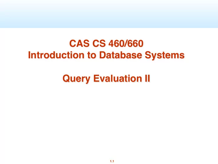
CAS CS 460/660 Introduction to Database Systems Query Evaluation II 1.1 Cost-based Query Sub-System Select * Queries From Blah B Where B.blah = blah Query Parser Query Optimizer Plan Plan Cost Catalog Manager Generator Estimator
1.1
1.2
Statistics
Schema
Select * From Blah B Where B.blah = blah
1.3
■ We will consider how to implement: ➹ Selection ( σ ) Selects a subset of rows from relation. ➹ Projection ( π ) Deletes unwanted columns from relation. ➹ Join ( ⋈ ) Allows us to combine two relations. ➹ Set-difference ( - ) Tuples in reln. 1, but not in reln. 2. ➹ Union ( ∪ ) Tuples in reln. 1 and in reln. 2. ➹ Also: Aggregation (SUM, MIN, etc.) and GROUP BY ■ Since each op returns a relation, ops can be composed ! After we cover the
them.
1.4
1.5
■ Similar to old schema; rname added for variation.
(assume pages of 4000 bytes each)
■ Reserves: ➹ Each tuple is 40 bytes long, 100 tuples per page, 1000 pages. (100K reseravtions) ■ Sailors: ➹ Each tuple is 50 bytes long, 80 tuples per page, 500 pages. (40K sailors)
Sailors (sid: integer, sname: string, rating: integer, age: real) Reserves (sid: integer, bid: integer, day: date, rname: string)
1.6
■ Of the form ■ Question: how best to perform? Depends on: ➹ what indexes/access paths are available ➹ what is the expected size of the result (in terms of number of tuples and/or number of pages) ■ Size of result approximated as
size of R * reduction factor
➹ “reduction factor” is usually called selectivity. ➹ estimate of reduction factors is based on statistics – we will discuss shortly.
SELECT * FROM Reserves R WHERE R.date > ‘1/1/2015’
value
.
1.7
■ With no index, unsorted: ➹ Must essentially scan the whole relation ➹ cost is M (#pages in R). For “Reserves” = 1000 I/Os. ■ With no index, sorted on day: ➹ cost of binary search + number of pages containing results. ➹ For reserves = 10 I/Os + ⎡ ⎡selectivity*1000⎤ ⎤ ■ With an index on selection attribute: ➹ Use index to find qualifying data entries, ➹ then retrieve corresponding data records. ➹ (Hash index useful only for equality selections.)
1.8
■ Cost depends on #qualifying tuples, and clustering. ➹ Cost:
➹ In example “Reserves” relation, if 10% of tuples qualify (result size estimate: 100 pages, 10000 tuples).
1.9
■ Important refinement for unclustered indexes:
looked at just once (though # of such pages likely to be higher than with clustering).
Index entries Data entries direct search for (Index File) (Data file) Data Records data entries Data entries Data Records
CLUSTERED UNCLUSTERED
1.10
■ Such selection conditions are first converted to conjunctive normal form
(CNF):
➹ (day<8/9/94 OR bid=5 OR sid=3 ) AND (rname=‘Paul’ OR bid=5 OR sid=3) ■ We only discuss the case with no ORs (a conjunction of terms of the form
attr op value).
■ A B-tree index matches (a conjunction of) terms that involve only
attributes in a prefix of the search key.
➹ Index on <a, b, c> matches a=5 AND b= 3, but not b=3. ■ For Hash index, must have all attributes in search key
☛ (day<8/9/94 AND rname=‘Paul’) OR bid=5 OR sid=3
1.11
1.12
■ Consider day < 8/9/94 AND bid=5 AND sid=3. ■ A B+ tree index on day can be used;
■ Similarly, a hash index on <bid, sid> could be used; ➹ Then, day<8/9/94 must be checked. ■ How about a B+tree on <rname,day>? ■ How about a B+tree on <day, rname>? ■ How about a Hash index on <day, rname>?
1.13
■ Second approach: if we have 2 or more matching indexes (w/
➹ Get sets of rids of data records using each matching index. ➹ Then intersect these sets of rids. ➹ Retrieve the records and apply any remaining terms.
■ Consider day<8/9/94 AND bid=5 AND sid=3. With a B+ tree
➹ Note: commercial systems use various tricks to do this: § bit maps, bloom filters, index joins
1.14
1.15
■ Joins are a very common query operation. ■ Joins can be very expensive: Consider an inner join of R and S each with 1M records. Q: How many tuples in the answer? (cross product in worst case, 0 in the best(?)) ■ Many join algorithms have been developed ■ Can have very different join costs.
1.16
■ In algebra: R ⋈ S. Common! Must be carefully optimized. R × S is
large; so, R × S followed by a selection is inefficient.
■ Assume: ➹ M = 1000 pages in R, pR =100 tuples per page. ➹ N = 500 pages in S, pS = 80 tuples per page. ➹ In our examples, R is Reserves and S is Sailors. ■ Cost metric : # of I/Os. We will ignore output costs. ■ We will consider more complex join conditions later.
SELECT * FROM Reserves R1, Sailors S1 WHERE R1.sid=S1.sid
1.17
■ For each tuple in the outer relation R, we scan the entire inner relation S. ■ How much does this Cost? ■ (pR * M) * N + M = 100,000*500 + 1000 I/Os. ( about 50M I/Os!!) ➹ At 10ms/IO, Total: ??? ■ What if smaller relation (S) was outer? ■ (ps * N) *M + N = 40,000*1000 + 500 I/Os. (better…. J 40M I/Os) ■ Prohibitively expensive…
foreach tuple r in R do foreach tuple s in S do if ri == sj then add <r, s> to result
1.18
■ For each page of R, get each page of S, and write out matching pairs of
tuples <r, s>, where r is in R-page and S is in S-page.
■ What is the cost of this approach? ■ M*N + M= 1000*500 + 1000 = 501000 ➹ If smaller relation (S) is outer, cost = 500*1000 + 500 = 500500
foreach page bR in R do foreach page bS in S do foreach tuple r in bR do foreach tuple s in bSdo if ri == sj then add <r, s> to result
1.19
■ Page-oriented NL doesn’t exploit extra buffers. ■ Alternative approach: Use one page as an input buffer for scanning
the inner S, one page as the output buffer, and use all remaining pages to hold ``block’’ of outer R.
■ For each matching tuple r in R-block, s in S-page, add <r, s> to
R & S
block of R tuples (k <= B-2 pages) Input buffer for S Output buffer
Join Result
1.20
■ Cost:
Scan of outer + #outer blocks * scan of inner
➹ #outer blocks = ceiling(#pages of outer/blocksize) ■ With Reserves (R) as outer, and 100 pages/Block (B=102): ➹ Cost of scanning R is 1000 I/Os; a total of 10 blocks (B=102). ➹ Per block of R, we scan Sailors (S); 10*500 I/Os. ➹ Total cost: 10*500+1000 = 6000 I/Os ➹ If space for just 90 pages of R, we would scan S 12 times. ■ With 100-page block of Sailors as outer: ➹ Cost of scanning S is 500 I/Os; a total of 5 blocks. ➹ Per block of S, we scan Reserves; 5*1000 I/Os. ➹ Total cost: 5 * 1000 + 500 = 5500 I/Os. (Much better J) ➹ We may be able to do even better for different B!
1.21
■ If there is an index on the join column of one relation (say S), can make it
the inner and exploit the index.
➹ Cost: M + ( (M*pR) * cost of finding matching S tuples) ■ For each R tuple, cost of probing S index is about 1.2 for hash index, 2-4
for B+ tree.
■ Cost of then finding S tuples (assuming Alt. (2) or (3) for data entries)
depends on clustering.
■ Clustered index: 1 I/O per page of matching S tuples. ■ Unclustered: up to 1 I/O per matching S tuple.
foreach tuple r in R do foreach tuple s in S where ri == sj do add <r, s> to result
1.22
■ Hash-index (Alt. 2) on sid of Sailors (as inner): ➹ Scan Reserves: 1000 page I/Os, 100*1000 tuples. ➹ For each Reserves tuple: 1.2 I/Os to get data entry in index, plus 1 I/O to get (the exactly one) matching Sailors tuple. Total: 1000+100*1000*2.2 ■ Hash-index (Alt. 2) on sid of Reserves (as inner): ➹ Scan Sailors: 500 page I/Os, 80*500 tuples. ➹ For each Sailors tuple: 1.2 I/Os to find index page with data entries, plus cost of retrieving matching Reserves tuples. Assuming uniform distribution, 2.5 reservations per sailor (100,000 / 40,000). Cost of retrieving them is 1
➹ Totals: 500 + 80*500*2.2 = 88.5K I/Os!!! (not so good here L) ➹ Other scenarios may be better though.
1.23
■ Sort R and S on the join column, then scan them to do a ``merge’’ (on
join col.), and output result tuples.
■ Particularly useful if ➹ one or both inputs are already sorted on join attribute(s) ➹ output is required to be sorted on join attributes(s) ■ “Merge” phase can require some back tracking if duplicate values appear in
join column
■ R is scanned once; each S group is scanned once per matching R tuple.
(Multiple scans of an S group will probably find needed pages in buffer.)
1.24
■ Cost: Sort S +Sort R + (M+N) ➹ The cost of merging: usually M+N, § worst case is M*N (but very unlikely!) ■ With 35, 100 or 300 buffer pages, both Reserves and Sailors can be sorted
in 2 passes; total join cost: 7500.
(BNL cost: 2500 to 16500 I/Os)
1.25
■ For B = 35 ➹ Sort-Merge: § sort R: in two passes=> 4M = 4000 § sort S: in two passes => 4N = 2000 § merge: M+N (hopefully…) => 1500 § Total: 7500 ➹ Block Nested Loop: § celing(N/B-2)*M+N = 16*1000+500 = 16500 ➹ Sort-Merge Better for B=35!!!! ■ For B = 300 ➹ Sort-Merge: the same: 7500 ➹ BNLJ: § celing(N/B-2)*M+N = 2*1000+500 = 2500 ➹ Here BNLJ is better!!!!
1.26
■ We can combine the merging phases in the sorting of R and S with the
merging required for the join.
➹ Pass 0 as before, but apply to both R then S before merge. ➹ If B > , where L is the size of the larger relation, using the sorting refinement that produces runs of length 2B in Pass 0, #runs of each relation is < B/2. ➹ In “Merge” phase: Allocate 1 page per run of each relation, and `merge’ while checking the join condition ➹ Cost: read+write each relation in Pass 0 + read each relation in (only) merging pass (+ writing of result tuples). ➹ In example, cost goes down from 7500 to 4500 I/Os for B=300. ■ In practice, the I/O cost of sort-merge join, like the cost of external sorting,
is linear.
1.27
■ If several operations are executing concurrently, estimating the number
■ Repeated access patterns interact with buffer replacement policy. ➹ e.g., Inner relation is scanned repeatedly in Simple Nested Loop Join. With enough buffer pages to hold inner, replacement policy does not matter. Otherwise, MRU is best, LRU is worst (sequential flooding). ➹ Does replacement policy matter for Block Nested Loops? ➹ What about Index Nested Loops? Sort-Merge Join?
1.28
■ Partition both relations
using hash function h.
■ R tuples in partition Ri
will only match S tuples in partition Si. For i= 1 to #partitions { Read in partition Ri and hash it using h2 (not h). Scan partition Si and probe hash table for matches. }
Partitions
Input buffer for Si
Hash table for partition Ri (k < B-1 pages)
B main memory buffers Disk
Output buffer
Disk Join Result
hash fn
h2
h2
B main memory buffers Disk Disk Original Relation
OUTPUT 2 INPUT 1 hash function
h
B-1
Partitions 1 2 B-1
1.29
■ #partitions k < B, and B-1 > size of smaller partition to be held in memory.
Assuming uniformly sized partitions, and maximizing k, we get:
k= B-1, and M/(B-1) < B-2, i.e., B must be > ■ Since we build an in-memory hash table to speed up the matching of
tuples in the second phase, a little more memory is needed.
■ If the hash function does not partition uniformly, one or more R partitions
may not fit in memory. Can apply hash-join technique recursively to do the join of this R-partition with corresponding S-partition.
1.30
■ In partitioning phase, read+write both relns; 2(M+N). In matching phase,
read both relns; M+N I/Os.
■ In our running example, this is a total of 4500 I/Os. ■ Sort-Merge Join vs. Hash Join: ➹ Given a minimum amount of memory (what is this, for each?) both have a cost
reln fits in memory). Also, Hash Join shown to be highly parallelizable. ➹ Sort-Merge less sensitive to data skew; result is sorted.
1.31
■ Intersection and cross-product special cases of join. ■ Union (Distinct) and Except similar; we’ll do union. ■ Sorting based approach to union: ➹ Sort both relations (on combination of all attributes). ➹ Scan sorted relations and merge them. ➹ Alternative: Merge runs from Pass 0 for both relations. ■ Hash based approach to union: ➹ Partition R and S using hash function h. ➹ For each S-partition, build in-memory hash table (using h2), scan corr. R- partition and add tuples to table while discarding duplicates.
1.32
■ Equalities over several attributes
(e.g., R.sid=S.sid AND R.rname=S.sname):
➹ For Index NL, build index on <sid, sname> (if S is inner); or use existing indexes on sid or sname. ➹ For Sort-Merge and Hash Join, sort/partition on combination of the two join columns. ■ Inequality conditions (e.g., R.rname < S.sname): ➹ For Index NL, need (clustered!) B+ tree index. § Range probes on inner; # matches likely to be much higher than for equality joins. ➹ Hash Join, Sort Merge Join not applicable! ➹ Block NL quite likely to be the best join method here.
1.33
■ Implementation of Relational Operations as Iterators ➹ Focus largely on External algorithms (sorting/hashing) ■ Choices depend on indexes, memory, stats,… ■ Joins ➹ Blocked nested loops: § simple, exploits extra memory ➹ Indexed nested loops: § best if 1 rel small and one indexed ➹ Sort/Merge Join § good with small amount of memory, bad with duplicates ➹ Hash Join § fast (if enough memory), bad with skewed data § Relatively easy to parallelize
1.34
1.35
■ Similar to old schema; rname added for variations. ■ Reserves: ➹ Each tuple is 40 bytes long, 100 tuples per page, 1000 pages. So, M = 1000, pR = 100. ■ Sailors: ➹ Each tuple is 50 bytes long, 80 tuples per page, 500 pages. ➹ So, N = 500, pS = 80.
Sailors (sid: integer, sname: string, rating: integer, age: real) Reserves (sid: integer, bid: integer, day: dates, rname: string)
1.36
■ Without grouping: ➹ In general, requires scanning the relation. ➹ Given a tree index whose search key includes all attributes in the SELECT or
WHERE clauses, can do index-only scan.
■ With grouping: ➹ Sort on group-by attributes, then scan relation and compute aggregate for each
➹ Similar approach based on hashing on group-by attributes. ➹ Given a tree index whose search key includes all attributes in SELECT,
WHERE and GROUP BY clauses, can do index-only scan; if group-by
attributes form prefix of search key, can retrieve data entries/tuples in group- by order.
1.37
■ The Sort iterator naturally permutes its input so that all tuples
are output in sequence
■ The Aggregate iterator keeps running info (“transition values”
Example transVals: ➹ For COUNT, it keeps count-so-far ➹ For SUM, it keeps sum-so-far ➹ For AVERAGE it keeps sum-so-far and count-so-far
■ As soon as the Aggregate iterator sees a tuple from a new
group:
function
E.g. for AVERAGE it returns (sum-so-far/count-so-far)
Sort Aggregate
1.38
Sort Aggregate
A B C D A B A
<A, 1> <B,1>
AB <B,2> B <A, 2> <A, 3>
C
1.39
■ The Hash iterator permutes its input so that all tuples are
■ The Aggregate iterator keeps running info (“transition values”
➹ E.g., for COUNT, it keeps count-so-far ➹ For SUM, it keeps sum-so-far ➹ For AVERAGE it keeps sum-so-far and count-so-far
■ When the Aggregate iterator sees a tuple from a new group:
function
E.g. for AVERAGE it returns (sum-so-far/count-so-far)
Hash Aggregate
1.40
■ Partition:
Each group will be in a single disk-based partition file. But those files have many groups inter-mixed.
■ Rehash:
For Each Partition i: hash i into an in-memory hash table Return results until records exhuasted then i+ +
B main memory buffers Disk Disk Original Relation
OUTPUT 2 INPUT 1 hash function
hp
B-1
Partitions 1 2 B-1
Partitions
Hash table for partition Ri (k < B pages)
B main memory buffers Disk Result
fn INPUT
hash function
h2p
1.41
■ Put summarization into the hashing process ➹ During the ReHash phase, don’t store tuples, store pairs of the form <GroupVals, TransVals> ➹ When we want to insert a new tuple into the hash table § If we find a matching GroupVals, just update the TransVals appropriately § Else insert a new <GroupVals,TransVals> pair ■ What’s the benefit? ➹ Q: How many pairs will we have to maintain in the rehash phase? ➹ A: Number of distinct values of GroupVals columns § Not the number of tuples!! ➹ Also probably “narrower” than the tuples HashAgg
1.42
■ Issue is removing duplicates. ■ Basic approach is to use sorting
➹ 1. Scan R, extract only the needed attrs (why do this 1st?) ➹ 2. Sort the resulting set ➹ 3. Remove adjacent duplicates ➹ Cost: Reserves with size ratio 0.25 = 250 pages. With 20 buffer pages can sort in 2 passes, so 1000 +250 + 2 * 2 * 250 + 250 = 2500 I/Os
■ Can improve by modifying external sort algorithm:
➹ Modify Pass 0 of external sort to eliminate unwanted fields. ➹ Modify merging passes to eliminate duplicates. ➹ Cost: for above case: read 1000 pages, write out 250 in runs of 20 pages, merge runs = 1000 + 250 +250 = 1500. SELECT DISTINCT
R.sid, R.bid
FROM Reserves R
1.43
■ If an index on the relation contains all wanted attributes in its search key,
can do index-only scan.
➹ Apply projection techniques to data entries (much smaller!) ■ If an ordered (i.e., tree) index contains all wanted attributes as prefix of
search key, can do even better:
➹ Retrieve data entries in order (index-only scan), discard unwanted fields, compare adjacent tuples to check for duplicates. ■ Same tricks apply to GROUP BY/Aggregation
1.44
■ Queries are composed of a few basic operators; ➹ The implementation of these operators can be carefully tuned (and it is important to do this!). ➹ Operators are “plug-and-play” due to the Iterator model. ■ Many alternative implementation techniques for each operator; no
universally superior technique for most.
■ Must consider alternatives for each operation in a query and
choose best one based on statistics, etc.
■ This is part of the broader task of Query Optimization, which we
will cover next!