[PPT] - Psychophysics, Estimating Perceptual Scales with Interval Properties PowerPoint Presentation

SLIDE 1

Estimating Perceptual Scales with Interval Properties

Kenneth Knoblauch & Laurence T. Maloney

1. Inserm, U846

Stem Cell and Brain Research Institute

Dept. Integrative Neurosciences

Bron, France

2. Department of Psychology

Center for Neural Science New York University New York, NY 10003, USA

Psychophysics, qu’est-ce que c’est ?

A body of techniques and analytic methods to study the relation between physical stimuli and the organism’s (classification) behavior to infer internal states of the

rganism or their organization.

Gustav Fechner (1801 - 1887)

Classical Psychophysical Paradigm Event

φi ∈ {φ1, · · · , φn}

Observer

ǫ ∼ i.i.d. ψj ∈ {ψ1, · · · , ψm} + ǫ

Pr(Rij) = f ({φi}; Ψ) , f is a Psychometric Function

1 2 3 4 0.0 0.2 0.4 0.6 0.8 1.0

Proportion Correct

Response

Rij ∈ {R11, R12, . . . , Rnp}

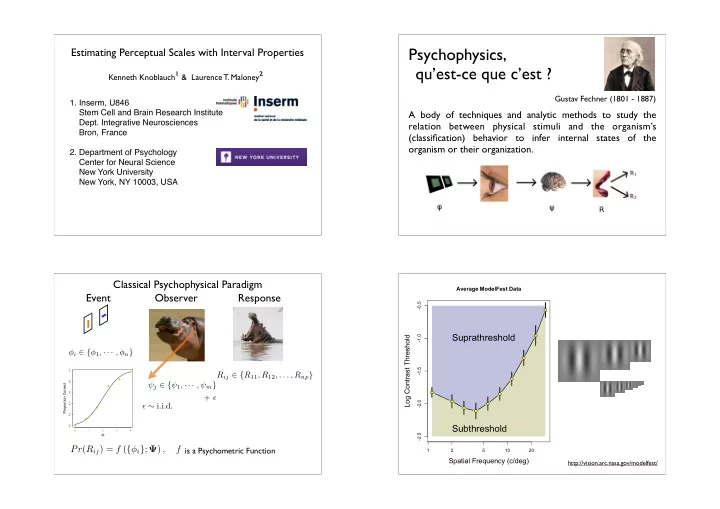
1 2 5 10 20

2.5
2.0
1.5
1.0
0.5

Average ModelFest Data

Spatial Frequency (c/deg) Log Contrast Threshold

Suprathreshold Subthreshold

http://vision.arc.nasa.gov/modelfest/

SLIDE 2

Paired Comparisons

a b Find numbers, such that when b is judged of higher contrast than a, .

(ψa, ψb), ψb > ψa

Decision variable:

∆ = ψb − ψa + ǫ, ǫ ∼ N(0, σ2) (ψ1, ψ2, . . . , ψn)

Only yields an ordinal scale! Any monotonic transformation of the above scale is equally valid!

Equal-variance, Gaussian Signal Detection Model

Series of Suprathreshold contrasts

How to quantify the evolution of suprathreshold perception along a physical dimension (like contrast)? How do different perceptual dimensions combine?

0.05 0.07 0.10 0.13 0.19 0.26 0.36 0.50 0.70

Two Questions to be considered in this talk 1) Difference Scaling: MLDS

(Maloney & Yang (2003). J Vision)

2) Conjoint Measurement: MLCM

(Luce & Tukey (1964) J Math Psych; Ho, Landy & Maloney (2008) Psych Science)

Both methods based on ordering intervals between stimuli and not on ordering stimuli, per se. Ordering intervals leads to scales with interval properties, i.e, equal scale differences correspond to equal perceptual differences. Methods that yield an interval scale

Knoblauch & Maloney, J. Stat. Soft., 25, 1 - 26.

Difference Scaling: Correlation in scatterplots

r = 0
r = 0.1
r = 0.2
r = 0.3
r = 0.4
r = 0.5
r = 0.6
r = 0.7
r = 0.8
r = 0.9
r = 0.98
0.0

0.2 0.4 0.6 0.8 1.0 0.0 0.2 0.4 0.6 0.8 1.0

r Difference Scale Value

ψ(r) ≈ r2

SLIDE 3

Difference Scaling: Triads

a b c

Between which pair, (a, b) or (b, c), is the contrast difference greatest?

Conjoint Measurement

Ho, Landy & Maloney (2008) Psych Science

Conjoint Measurement is a psychophysical procedure used to estimate the interaction of perceptual scales for stimuli distributed along physical continua. n ≥ 2 Luce & Tukey (1964) J Math Psych

TIME Fixation 200ms Surface 1 400ms ISI (blank screen) 200ms Surface 2 400ms Response

!"#$!%&'()&'+, !"#$!%&'()&'+,

From a set of p stimuli varying along 2 dimensions, a random pair, , is chosen and presented to the observer as in this example. Which is bumpier (glossier)? (Iij, Ikl) The aim of the Maximum Likelihood Difference Scaling (MLDS) procedure is to estimate scale values, that best capture the observer’s judgments of the perceptual difference between the stimuli in each pair.

Maximum Likelihood Difference Scaling: MLDS The decision model

where are estimated scale values, and a scale factor. ψi σ Given a quadruple, from a single trial, we assume that the observer chooses the upper pair to be further apart when q = (a, b ; c, d), ǫ ∼ N(0, σ2)

∆(a, b ; c, d) = (ψd − ψc) − (ψb − ψa) + ǫ > 0

SLIDE 4

B1 = ψb(b1) + χg(g1) B2 = ψb(b2) + χg(g2) ∆ = B1 − B2 + ǫ > 0 ⇔ “First” ǫ ∼ N(0, σ2)

Ho, Landy & Maloney (2008), Psych Science

The decision model

b2 g2 b1 g1 Bumpier? Maximum Likelihood Conjoint Measurement: MLCM Estimation of Scale Values: MLDS

L(Ψ, σ) =

n

k=1

Φ

δ
qk

σ 1−Rk 1 − Φ

δ
qk

σ Rk

Maloney and Yang (2003) used a direct method for estimating

the maximum likelihood scale values, where δ(qk) = |ψd − ψc| −| ψb − ψa| Φ Rk Ψ =( ψ2, ψ3, . . . , ψp−1) is the cumulative standard Gaussian (a probit analysis) is 0/1 if the judgment is lower/upper ψ1 = 0, ψp = 1 for identifiability, p − 1 leaving parameters to estimate

Maloney LT, Yang JN (2003). “Maximum Likelihood Difference Scaling.” Journal of Vision, 3(8), 573–585. URL http://www.journalofvision.org/3/8/5.

Estimation of Scale Values: MLCM

Ho, Landy & Maloney (2008) used a direct method for estimating the maximum likelihood scale values, L(Ψ, σ) =

n

k=1

Φ

δ
qk

σ 1−Rk 1 − Φ

δ
qk

σ Rk

where

Ψ = (ψ2, · · · , ψp, χ2, · · · , χq) δ(qk) = (ψb1 + χg1) − (ψb2 + χg2)

Φ Rk is the cumulative standard Gaussian (a probit analysis) is 0/1 if the judgment is left/right image

ψ1 = χ1 = 0

and for identifiability, leaving parameters to estimate

σ = 1 p + q − 2

Estimation of Scale Values: MLDS

This problem can, also, be conceptualized as a GLM. Each level of the stimulus is treated as a covariate in the design matrix, taking on values of , depending on the presence of the stimulus in a trial and its weight in the decision variable. 0 or ± 1 For model identifiability, we drop the first column (fixing and ), equal variance, Gaussian, signal detection model. ψ1 = 0 σ = 1

p p p p p p p p p p p

The estimated scale is unique up to linear transformations.

resp S1 S2 S3 S4 1 4 8 2 3 2 1 2 3 6 11 3 1 2 6 7 10 4 4 11 1 2 5 9 11 7 8 6 7 10 1 3         1 −1 −1 1 1 −1 −1 1 1 −1 −1 1 1 −1 −1 1 1 −1 −1 1 1 −1 −1 1        

. . . . . .

SLIDE 5

Estimation of Scale Values: MLCM

The problem can also be conceptualized as a GLM. Each level of the stimulus is treated as a covariate in the model matrix, taking on values of in the design matrix, depending on the presence of the stimulus in a trial and its weight in the decision variable. 0 or ± 1 For model identifiability, we drop the first two columns along each dimension, fixing and .

Resp G1 G2 B1 B2 1 1 3 4 4 3 2 1 3 5 4 2 3 0 1 1 1 4 4 0 2 3 1 2 5 0 1 4 3 4 6 1 1 5 5 2

p p p p p q q q q q         1 −1 −1 1 1 −1 −1 1 1 −1 1 −1 1 −1 1 −1 1 −1 1 −1 −1 1        