
SLIDE 1
1
Pri rinciples nciples of
- f Com
- mmunications
munications
EC ECS S 332 32
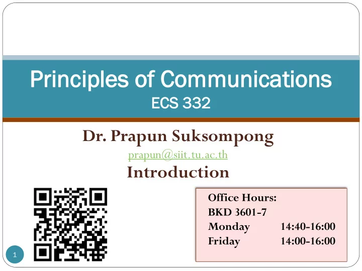
- Dr. Prapun Suksompong
Pri rinciples nciples of of Com ommunications munications EC - - PowerPoint PPT Presentation
Pri rinciples nciples of of Com ommunications munications EC ECS S 332 32 Dr. Prapun Suksompong prapun@siit.tu.ac.th Introduction Office Hours: BKD 3601-7 Monday 14:40-16:00 Friday 14:00-16:00 1 Course Organization Course
1
2
Course Website:
Lectures:
Wednesday 09:00-10:20 BKD 3206 Friday
10:40-12:00 BKD 3206
Textbook: Communication Systems: An Introduction to
By A. Bruce Carlson and Paul B. Crilly 5th International edition Call No. TK5102.5 C3 2010 ISBN: 978-007-126332-0
1
3
Shannon, Claude. A Mathematical Theory Of
4
1938 MIT master's thesis: A Symbolic
Insight: The binary nature of Boolean
logic was analogous to the ones and zeros used by digital circuits.
The thesis became the foundation of
practical digital circuit design.
The first known use of the term bit to
refer to a “binary digit.”
Possibly the most important, and also the
most famous, master's thesis of the century.
It was simple, elegant, and important.
5
1948: A Mathematical
Theory of Communication
Bell System Technical Journal,
October, 1948.
September 1949: Book
Create the architecture and
concepts governing digital communication.
Invent Information Theory:
Simultaneously founded the subject, introduced all of the major concepts, and stated and proved all the fundamental theorems.
6
Link posted in the
[An offprint from the Bell System Technical Journal]
7
[http://www.youtube.com/watch?v=z2Whj_nL-x8]
8
Claude E. Shannon (1972) David S. Slepian (1974) Robert M. Fano (1976) Peter Elias (1977) Mark S. Pinsker (1978) Jacob Wolfowitz (1979) W . Wesley Peterson (1981) Irving S. Reed (1982) Robert G. Gallager (1983) Solomon W . Golomb (1985) William L. Root (1986) James L. Massey (1988) Thomas M. Cover (1990) Andrew J. Viterbi (1991) Elwyn R. Berlekamp (1993) Aaron D. Wyner (1994)
Imre Csiszár (1996) Jacob Ziv (1997) Neil J. A. Sloane (1998) Tadao Kasami (1999) Thomas Kailath (2000) Jack Keil Wolf (2001) Toby Berger (2002) Lloyd R. Welch (2003) Robert J. McEliece (2004) Richard Blahut (2005) Rudolf Ahlswede (2006) Sergio Verdu (2007) Robert M. Gray (2008) Jorma Rissanen (2009) Te Sun Han (2010) Shlomo Shamai (Shitz) (2011)
9
1.
2.
3.
10
Information source: produce a message Transmitter: operate on the message to create a signal
Noise Source
Receiver
Transmitter Information Source
Destination
Channel
Received Signal Transmitted Signal Message Message
11
Channel: the medium over which the signal, carrying the
Receiver: transform the signal back into the message
Noise Source
Receiver
Transmitter Information Source
Destination
Channel
Received Signal Transmitted Signal Message Message
12
Destination: a person or a machine, for whom or which
Noise Source
Receiver
Transmitter Information Source
Destination
Channel
Received Signal Transmitted Signal Message Message
13
010100 010100 Binary Interface
Take the bits from one place to another. Binary data stream (sequence of data) without meaning (from channel viewpoint). This is the major layering of all digital communication systems. Know the probabilistic structure of the input source. + noise & interference Waveform sequence symbols bits
14
A Brief History of Communications: IEEE
ประวัติย่อ "การสื่อสารโลก": ห้าสิบปีชมรมไฟฟ้า
สื่อสาร—รากฐานสู่อนาคต
Thai Telecommunications Encyclopedia
Links posted in the “references” section of
1
Office Hours: BKD 3601-7 Monday 14:40-16:00 Friday 14:00-16:00
2
3
4
5
6
Human Audiogram (Audibility Curve) [http://psyc254.uconn.edu/Lecture18/]
Approximate best frequencies of various places along the basilar membrane, in hertz. Schematic showing the cochlea unrolled, in cross-section.
[Schnupp, Nelken, and King, 2010, Fig 2.2] [Schnupp, Nelken, and King, 2010, Fig 2.1] [Schnupp, Nelken, and King, 2010, Fig 2.2]
The cochlea has sometimes been described as a biological Fourier analyzer.
7
1 0, c t A t T
1 2 3 4 5 0.2 0.4 0.6 0.8 1 f [Hz]
C f
A T t
1, 1 A T
t A
m = [-1,-1,1,-1,-1,1,1,-1,-1,-1,1,-1,-1,1,-1,1,1,-1,-1,-1,-1,1,-1,-1,-1,-1,-1,1,-1,1]
s t
Can you sketch the spectrum of s(t)?
8
1 0, c t A t T
1 2 3 4 5 0.2 0.4 0.6 0.8 1 f [Hz]
C f
A T t
1, 1 A T
t A
m = [-1,-1,1,-1,-1,1,1,-1,-1,-1,1,-1,-1,1,-1,1,1,-1,-1,-1,-1,1,-1,-1,-1,-1,-1,1,-1,1]
s t
1 n k k
s t m c t kT
This is also the spectrum of for any . c t kT k
9
1 0, c t A t T
1 2 3 4 5 0.2 0.4 0.6 0.8 1 f [Hz]
C f
A T t
1, 1 A T
t A
m = [-1,-1,1,-1,-1,1,1,-1,-1,-1,1,-1,-1,1,-1,1,1,-1,-1,-1,-1,1,-1,-1,-1,-1,-1,1,-1,1]
s t
1 n k k
s t m c t kT
1 2 n j fkT k k
S f C f m e
This is also the spectrum of for any . c t kT k
10
1 1 2 n n j fkT k k k k
s t m c t kT S f C f m e
1 0, c t A t T
1 2 3 4 5 2 4 6 8 10 f [Hz]
1 2 3 4 5 0.2 0.4 0.6 0.8 1 f [Hz]
C f
S f
A T t
1, 1 A T
t A
m = [-1,-1,1,-1,-1,1,1,-1,-1,-1,1,-1,-1,1,-1,1,1,-1,-1,-1,-1,1,-1,-1,-1,-1,-1,1,-1,1]
s t
This is also the spectrum of for any . c t kT k
11
12
2 2 2 2 2
1 1 cos 2 2 2 cos sin 2cos 1 cos 2 2sin 1 cos 2 1 1 cos 2 2 2
j ft j j j j ft j f t c c c c c c
G f e j x x x x g t t e G f e g g t e dt f t f t G f f m t f t M f f f f e f f f M e
(Will be provided on the midterm)
1
Office Hours: BKD 3601-7 Monday 14:40-16:00 Friday 14:00-16:00
2
Modulation:
1 1 cos 2 2 2
c c c
m t f t M f f M f f
Shifting Properties:
2 j ft
g t t e G f
2 j f t
e g t G f f
3
5 10
0.5 1 1.5
5 10
0.5 1 1.5
𝑦 𝑢 = cos 𝑢 − 1 3 cos 3𝑢 + 1 5 cos 5𝑢 𝑦 𝑢 𝑧 𝑢 = ℎ 𝑢 ∗ 𝑦(𝑢) ℎ 𝑢
4
5 10
0.5 1 1.5
5 10
0.5 1 1.5
5 10
0.5 1 1.5
5 10
0.5 1 1.5
𝑦 𝑢 = cos 𝑢 − 1 3 cos 3𝑢 + 1 5 cos 5𝑢 𝑧 𝑢 = 1 2 cos 𝑢 − 1 3 cos 3𝑢 + 1 5 cos 5𝑢
5
5 10
0.5 1 1.5
5 10
0.5 1 1.5
5 10
0.5 1 1.5
5 10
0.5 1 1.5
𝑦 𝑢 = cos 𝑢 − 1 3 cos 3𝑢 + 1 5 cos 5𝑢 𝑧 𝑢 = cos 𝑢 − 1 3 cos 3𝑢 + 1 2 1 5 cos 5𝑢
6
5 10
0.5 1 1.5
5 10
0.5 1 1.5
5 10
0.5 1 1.5
5 10
0.5 1 1.5
𝑦 𝑢 = cos 𝑢 − 1 3 cos 3𝑢 + 1 5 cos 5𝑢 𝑧 𝑢 = cos 𝑢 + 2 − 1 3 cos 3𝑢 + 2 + 1 5 cos 5𝑢 + 2 Components of the distorted signal all attain maximum or minimum values at the same time.
Surprising fact: an untrained human ear is curiously insensitive to phase distortion. The waveforms above would sound just about the same when driving a loudspeaker. Thus, phase distortion is seldom of concern in voice and music transmission.
7
5 10
0.5 1 1.5
5 10
0.5 1 1.5
5 10
0.5 1 1.5
5 10
0.5 1 1.5
𝑦 𝑢 = cos 𝑢 − 1 3 cos 3𝑢 + 1 5 cos 5𝑢 Same as time-shift!
1 1 cos cos 3 3 cos 5 5 2 3 2 5 2 1 1 cos cos 3 cos 5 2 3 2 5 2 2 y t t t t t t t x t
8
In a wireless mobile communication system, a transmitted
We refer to this phenomenon as multipath propagation
We call this fluctuation multipath fading. Remark: Reflections due to mismatched impedance on a cable system produce the same effect
9
10
v i i i
r t x t h t n t x t n t
v i i i
h t t
1
0.5 0.2 0.2 0.3 0.3 0.1 0.5
s s s
h t t t T t T t T
2
0.5 0.2 0.7 0.3 1.5 0.1 2.3
s s s
h t t t T t T t T
The signal received consists of a number of reflected rays, each characterized by a different amount of attenuation and delay.
ISI (Intersymbol Interference)
11
0.5 1 1.5 2 2.5 3 3.5 4 4.5 5 0.5 1 1.5 f |H1(f)| 0.5 1 1.5 2 2.5 3 3.5 4 4.5 5 0.5 1 f |P(f)| 0.5 1 1.5 2 2.5 3 3.5 4 4.5 5 0.5 1 1.5 f |H2(f)|
The transmitted signal (envelope) Channel with weak multipath Channel with strong multipath
1
[Gosling , 1999, Fig 1.1]
c f
Wavelength Frequency
8
3 10 m/s
2
Commercially exploited bands c f
Wavelength Frequency
8
3 10 m/s
[http://www.britannica.com/EBchecked/topic-art/585825/3697/Commercially-exploited-bands-of-the-radio-frequency-spectrum]
Note that the freq. bands are given in decades; the VHF band has 10 times as much frequency space as the HF band.
3
All cellular phone networks worldwide use a portion of the radio
frequency spectrum designated as ultra high frequency (UHF) (300 MHz to 3 GHz)
The UHF band is also used for television, Wi-Fi and Bluetooth
transmission.
Due to historical reasons, radio frequencies used for cellular
networks differ in the Americas, Europe, and Asia.
Frequency bands recommended by ITU-R (in June 2003) for
terrestrial Mobile telecommunication IMT-2000:
806-960 MHz 1710-2025 MHz 2110-2200 MHz 2500-2690 MHz
4
Efficiency of an antenna in radiating radio energy is
Too low frequency = too large antenna
Ex. The “Sanguine” submarine communication system
30 Hz (10,000 km wavelength) Designed (but never built) for the US Navy Base antenna: 24 km square mesh of wires. 10MW RF input
Radiate only 147 W All the remainder of the power dissipates as heat.
[Gosling, 1999, p 11]
5
Atmospheric absorption Quasi-optical propagation
Short wavelength = Deep
shadows behind obscuring
coverage.
Increased absorption by
[Gosling , 1999, Fig 1.1]
14 dB/km @ 60 GHz Make commu. very dependent on weather conditions
(terrestrial propagation)
6
7
http://www.ntc.or.th/uploadfiles/freq_chart_thai.htm
8
Spectral resource is limited. Most countries have government agencies responsible for
allocating and controlling the use of the radio spectrum.
Commercial spectral allocation is governed
globally by the International Telecommunications Union (ITU)
ITU Radiocommunication Sector (ITU-R) is responsible for radio
communication. in the U.S. by the Federal Communications Commission (FCC) in Europe by the European Telecommunications Standards Institute
(ETSI)
in Thailand by the National Telecommunications Commission
(NTC; คณะกรรมการกิจการโทรคมนาคมแห่งชาติ; กทช.)
replaced by the National Broadcasting and Telecommunications Commission
(NBTC; คณะกรรมการกิจการกระจายเสียง กิจการโทรทัศน์และกิจการโทรคมนาคมแห่งชาติ ; กสทช.)
Blocks of spectrum are now commonly assigned through spectral
9
Spectrum Wars: The Policy and
[Manner, 2003]
10
In Jan 2011, the FCC recently granted a conditional waiver to
LightSquared allowing the expansion of terrestrial use (for launching a new LTE network) of the mobile satellite spectrum (MSS) immediately neighboring that of the GPS
As its name suggested, MSS has been reserved for satellite services Earlier, FCC permitted “ancillary” terrestrial uses intended to “fill in”
locations where satellite coverage was problematic.
The new order allows a high powered nationwide terrestrial
broadband network.
Extremely high-powered ground-based transmissions could
potentially cause severe interference to GPS receivers.
LightSquared bought the spectrum right next door to GPS
cheaply, hoping to change the rules and make the spectrum more valuable.
[GPS World, December 2011]
11
RNSS L1 L1
12
GPS receivers have filters that do not block signals from the
These filters has enabled both low-cost and high-precision
Assumption: Signals in MSS band were low-power.
13
Spectrum is a scarce resource. Spectrum is allocated in “chunks” in frequency domain.
“Chunks” are licensed to (cellular/wireless) operators.
Within a single cellular operator, the chunk is further divided
Each channel has its own band of frequency.
1
2
1 2 3 4 5 6 7 8 9
0.5 1 Seconds
0.5 1 1.5 2 2.5 x 10
40.1 0.2 0.3 0.4 Frequency [Hz] Magnitude 1 2 3 4 5 6 7 8 9
1 2 Seconds
0.5 1 1.5 2 2.5 x 10
40.1 0.2 0.3 0.4 Frequency [Hz] Magnitude 1 2 3 4 5 6 7 8 9
0.5 1 Seconds
0.5 1 1.5 2 2.5 x 10
40.05 0.1 0.15 0.2 Frequency [Hz] Magnitude 1 2 3 4 5 6 7 8 9
0.5 1 Seconds
0.5 1 1.5 2 2.5 x 10
40.1 0.2 0.3 0.4 Frequency [Hz] Magnitude
3
1 2 3 4 5 6 7 8 9
0.5 1 Seconds
0.5 1 1.5 2 2.5 x 10
40.1 0.2 0.3 0.4 Frequency [Hz] Magnitude 1 2 3 4 5 6 7 8 9
0.5 1 Seconds
0.5 1 1.5 2 2.5 x 10
40.05 0.1 0.15 0.2 Frequency [Hz] Magnitude 1 2 3 4 5 6 7 8 9
1 2 Seconds
0.5 1 1.5 2 2.5 x 10
40.05 0.1 0.15 0.2 Frequency [Hz] Magnitude 1 2 3 4 5 6 7 8 9
0.5 Seconds
0.5 1 1.5 2 2.5 x 10
40.05 0.1 0.15 0.2 Frequency [Hz] Magnitude
4
1 1.0005 1.001 1.0015 1.002 1.0025 1.003 1.0035 1.004 1.0045 1.005
0.5 Seconds
0.5 1 1.5 2 2.5 x 10
40.1 0.2 0.3 0.4 Frequency [Hz] Magnitude 1 1.0005 1.001 1.0015 1.002 1.0025 1.003 1.0035 1.004 1.0045 1.005
0.5 Seconds
0.5 1 1.5 2 2.5 x 10
40.1 0.2 0.3 0.4 Frequency [Hz] Magnitude 1 1.0005 1.001 1.0015 1.002 1.0025 1.003 1.0035 1.004 1.0045 1.005
0.5 1 Seconds
0.5 1 1.5 2 2.5 x 10
40.05 0.1 0.15 0.2 Frequency [Hz] Magnitude 1 1.0005 1.001 1.0015 1.002 1.0025 1.003 1.0035 1.004 1.0045 1.005
0.5 Seconds
0.5 1 1.5 2 2.5 x 10
40.1 0.2 0.3 0.4 Frequency [Hz] Magnitude
(Zoomed in)
1
2
2 1
cos 2 x t t t
1 2 3 4 1 0.5 0.5 1 1 1 x1 t ( ) 4 t
At t = 2, frequency = ?
3
2 1
cos 2 x t t t
1 2 3 4 1 0.5 0.5 1 1 1 x1 t ( ) 4 t
At t = 2, f = t2 = 4 Hz?
cos 2 ft
Correct?
4
2 1
cos 2 x t t t
1 2 3 4 1 0.5 0.5 1 x1 t ( ) cos 2 4 t ( ) t
Correct? At t = 2, f = t2 = 4 Hz?
cos 2 ft
5
2 1
cos 2 x t t t
4 Hz is too low!!!
1 2 3 4 1 0.5 0.5 1 x1 t ( ) cos 2 4 t ( ) t 1.9 2 2.1 1 0.5 0.5 1 x1 t ( ) cos 2 4 t ( ) t
6
2 1
cos 2 x t t t
12 Hz?
1 2 3 4 1 0.5 0.5 1 x1 t ( ) cos 2 12 t ( ) t 1.9 2 2.1 1 0.5 0.5 1 x1 t ( ) cos 2 12 t ( ) t
7
Message signal Unmodulated carrier Phase-modulated signal Frequency-modulated signal
8
FM
x t
PM
x t
Remark: To see xPM(t) of time varying m(t), it is usually easier to look at the instantaneous freq. via the derivative first.
9
Message signal Unmodulated carrier Phase-modulated signal Frequency-modulated signal
10
11
FM
x t
PM
x t