SLIDE 2 2
Estimating Radiance
The reflected radiance is given by: The last term has dA while we are tracing
single photons and not fluxes.
' ) ' , )( ' , ( ) , ' , ( ) , ( w d w n w x L w w w f w x L
x i
Ω
= dA A w n w x L
i x i
) ( ) ' , )( ' , ( Φ =
∆ ∆Φ ≈
p p p
A w w x f w x L ) , ' , ( ) , (
Solution: Look at a circle
around x with radius r.
Add only photons
from that are
dA = pi * r Or weighted sum
(Gaussian kernel)
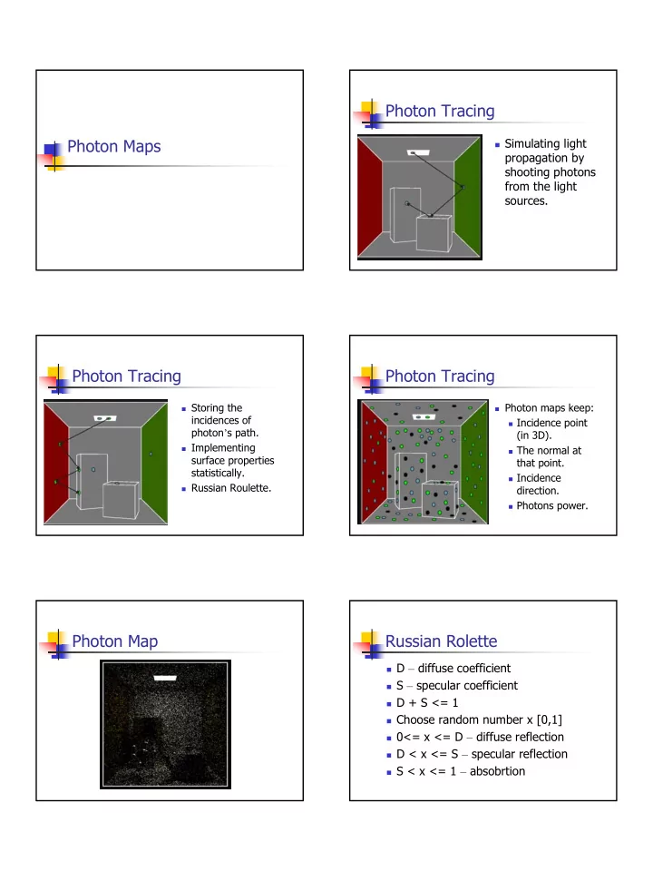
Building Photon Maps
Caustic Maps: Cast rays from light source toward
specular objects
Bias the sampling with “projection maps” that suggest good
places to send rays
Stop when the ray hits a diffuse surface, and store the point,
direction, intensity
When all the rays have been cast, build a kd-tree on the
points
Only need tree for later look-up, so worth building a good tree
Global Photon Map: Monte-Carlo Path tracing from
lights
Deposit a photon at every surface hit Use Russian Roulette to control cost and reduce bias
Producing the Image
Use ray tracing to determine the visible points Radiance at a point is broken into several
components:
One-bounce light from sources Light reflected specularly from other points Diffusely reflected caustics Light reflected diffusely multiple times
Each component is determined separately
Accurate method for directly seen light and “difficult”
geometry
Approximate for diffusely reflected light (low weight)
Computing Contributions
Direct illumination:
Accurate: Photon map gives approx. shadow, cast ray if not
certain
Approximate: Use diffuse photon map directly
Specular reflection:
Distribution ray tracing with importance
Caustics:
Use caustics photon map directly
Soft indirect illumination:
Accurate: “Radiance” style estimate Approximate: Global photon map
The “2 pass” algorithm
Step I: Building photon maps. Contains: direct,indirect,caustics photons. Step II: Rendering the scene using ray tracing. Direct lighting – sending rays to light sources. Specular – sending rays towards reflected direction. Caustics – from PM. Indirect – from PM.