Phase Type distributions Today: Phase type distribuions - PowerPoint PPT Presentation

Phase Type distributions Today: ◮ Phase type distribuions Distributions of phase type ◮ Definition ◮ Basic properties ◮ Closure properties Bo Friis Nielsen 1 Next week 1 DTU Informatics ◮ Phase type distributions ◮ Conditional Expectation, Martingales 02407 Stochastic Processes 8, October 29, 2013 Two weeks from now ◮ Brownian motion Bo Friis Nielsen Distributions of phase type Bo Friis Nielsen Distributions of phase type 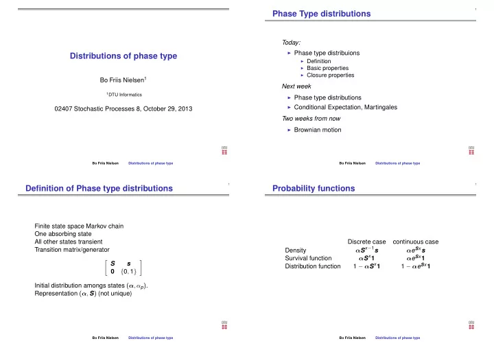Definition of Phase type distributions Probability functions Finite state space Markov chain One absorbing state All other states transient Discrete case continuous case α S x − 1 s Transition matrix/generator α e S x s Density α S x 1 α e S x 1 Survival function � S � s 1 − α S x 1 1 − α e S x 1 Distribution function { 0 , 1 } 0 Initial distribution amongs states ( α , α p ) . Representation ( α , S ) (not unique) Bo Friis Nielsen Distributions of phase type Bo Friis Nielsen Distributions of phase type

Addition of PH distributed random variables Minimum of PH Distributed random variables X ∼ PH ( α , S ) , Y ∼ PH ( β , T ) X ∼ PH ( α , S ) , Y ∼ PH ( β , T ) Z = X + Y � S Z = min ( X , Y ) � s β = L State space of dimension p 1 × p 2 0 T Combination of two independent chains thus Z ∼ PH ( γ , L ) with γ = ( α , α p 1 + 1 β ) Bo Friis Nielsen Distributions of phase type Bo Friis Nielsen Distributions of phase type Kronecker product Then A ⊗ B , A ⊗ I and I ⊗ B is given by   2 · 13 2 · 4 7 · 13 7 · 4 1 · 13 1 · 4 2 · 0 2 · 17 7 · 0 7 · 17 1 · 0 1 · 17   A ⊗ B =   3 · 13 3 · 4 5 · 13 5 · 4 11 · 13 11 · 4   3 · 0 3 · 17 5 · 0 5 · 17 11 · 0 11 · 17   a 11 B a 12 B a 1 k B . . . a 21 B a 22 B . . . a 2 k B  2 0 0 7 0 0 1 0 0    A ⊗ B = (1)  . . .  0 2 0 0 7 0 0 1 0 . . .   . . . . . .       0 0 2 0 0 7 0 0 1 a ℓ 1 B a ℓ 2 B . . . a ℓ k B   A ⊗ I =   3 0 0 5 0 0 11 0 0   Consider the matrices A , B , and I given by:   0 3 0 0 5 0 0 11 0   0 0 3 0 0 5 0 0 11 � 2 � 13   1 0 0 � � 7 1 4  13 4 0 0 0 0   . A = , B = , I = 0 1 0  3 5 11 0 17 0 17 0 0 0 0 0 0 1     0 0 13 4 0 0   I ⊗ B = .   0 0 0 17 0 0     0 0 0 0 13 4   0 0 0 0 0 17 Bo Friis Nielsen Distributions of phase type Bo Friis Nielsen Distributions of phase type

Minimum of PH Distributed Random Variables Maximum of PH Distributed random variables Z = max ( X , Y ) In the continuous case we get Z = min ( X , Y ) Z ∼ PH ( γ , L )   S ⊗ I + I ⊗ T I ⊗ t s ⊗ I � L = 0 S 0 S ⊗ T discrete case   L = 0 0 T S ⊗ I + I ⊗ T continuous case γ = α ⊗ β with obvious modifications for the transition probability matrix in the discrete case. The initial probability distribution is γ = ( α ⊗ β , α · β p 2 + 1 , α p 1 + 1 · β ) . Bo Friis Nielsen Distributions of phase type Bo Friis Nielsen Distributions of phase type Random sum of continuous PH distributed Expectation random variables Discrete case: ∞ S i = ( I − S ) − 1 = U � X ∼ PH ( α , S ) , Y i ∼ PH ( β , T ) where X is a discrete random variable and Y i are continuous random variables. i = 0 Continuous case X � � ∞ Z = Y i e S x d x = ( − S ) − 1 = U i = 0 0 Z ∼ PH ( γ , L ) with The ( i , j ) th element of U is the expected time spent in stat j before absorption, conditioned on initialization in state i . L = T ⊗ I + S ⊗ t β E ( X ) = α U 1 γ = α ⊗ β Bo Friis Nielsen Distributions of phase type Bo Friis Nielsen Distributions of phase type

The PH renewal process Residual life time and age distribution A finite state irreducible Markov chain. Q = S + ( 1 − α p + 1 ) − 1 s α � 1 discrete case π Q = Renewal density (assuming α p + 1 = 0) 0 continuous case h ( x ) = α e Q x s π ∼ = α U π = α U ( α U 1 ) − 1 Renewal function (assuming α p + 1 = 0) Residual life time and age in a stationary PH renewal process x βν ( S + s α − νπ ) − 1 s � I − e ( S + s α ) x � H ( x ) = − β is PH ( π , S ) distributed α S − 2 s x βν ( Q − νπ ) − 1 s � I − e Q x � = − β α S − 2 s Bo Friis Nielsen Distributions of phase type Bo Friis Nielsen Distributions of phase type Moment generating functions Moments By differentation of the moment generating functions we get α p + 1 + α ( I − e θ S ) − 1 s � discrete case � e θ X � E = α p + 1 + α ( I − θ ( − S ) − 1 ) − 1 1 continuous case � X i � = α i ! U i 1 E continuous case For the discrete case it is more common to use the generating E ( X ( X − 1 ) . . . ( X − i + 1 )) = α i ! U i S i − 1 1 discrete case function � z X � = α p + 1 + α ( I − z S ) − 1 s E Bo Friis Nielsen Distributions of phase type Bo Friis Nielsen Distributions of phase type