Ph.D. course in epidemiology: Fall 2012. Confounding Analysis of - - PowerPoint PPT Presentation

Ph.D. course in epidemiology: Fall 2012. Analysis of cohort studies. C & H, Ch. 6, 14-15. 18 September 2012

www.biostat.ku.dk/~nk/epiE12 Per Kragh Andersen

1

Confounding

• Epidemiology relies on observational studies or experiments of

nature

• Often these are poor experiments

— no control for confounding by extraneous influences

• Definition:

A confounder is a variable whose influence we would have controlled if we had been able to design the natural experiment.

2

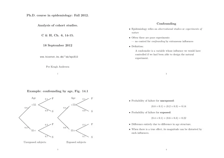
Example: confounding by age, Fig. 14.1

• ❅

❅ ❅ ❅ ❅

0.8 0.2

✟✟✟✟✟ ❍❍❍❍❍

0.1 0.9

✟✟✟✟✟ ❍❍❍❍❍

0.3 0.7

Age <55 55+ F S F S Unexposed subjects

• ❅

❅ ❅ ❅ ❅

0.4 0.6

✟✟✟✟✟ ❍❍❍❍❍

0.1 0.9

✟✟✟✟✟ ❍❍❍❍❍

0.3 0.7

Age <55 55+ F S F S Exposed subjects

3

• Probability of failure for unexposed:

(0.8 × 0.1) + (0.2 × 0.3) = 0.14

• Probability of failure for exposed:

(0.4 × 0.1) + (0.6 × 0.3) = 0.22

• Difference entirely due to difference in age structure.
• When there is a true effect, its magnitude can be distorted by

such influences.

4

Confounding when RR = 2

• ❅

❅ ❅ ❅ ❅

0.8 0.2

✟✟✟✟✟ ❍❍❍❍❍

0.1 0.9

✟✟✟✟✟ ❍❍❍❍❍

0.2 0.8

Age <55 55+ F S F S Unexposed subjects

• ❅

❅ ❅ ❅ ❅

0.4 0.6

✟✟✟✟✟ ❍❍❍❍❍

0.2 0.8

✟✟✟✟✟ ❍❍❍❍❍

0.4 0.6

Age <55 55+ F S F S Exposed subjects

5

Results.

• The true relative risk, RRT = 0.2/0.1 = 0.4/0.2 = 2
• Probability of failure for unexposed:

(0.8 × 0.1) + (0.2 × 0.2) = 0.12

• Probability of failure for exposed:

(0.4 × 0.2) + (0.6 × 0.4) = 0.32

• The apparent relative risk:

RRO = 0.32/0.12 = 2.67

6

Confounding

A confounder is:

• associated with outcome:

e.g., older persons have higher disease probability,

• associated with the exposure:

e.g., older persons are more / less likely to be exposed,

• not a result of exposure, i.e. not an intermediate variable.

Not a statistical property; cannot be seen from tables; common sense is required!

7

Confounding: schematically.

A variable C is a potential confounder for the relation: E → O if it is

• 1) related to the exposure:

E − C

• 2) an independent risk factor for the outcome:

C → O

• 3) not a consequence of the exposure:

E → C → O That is: E − C ց ւ O

8

Confounding.

The problem is that we do not always get a fair comparison between exposed and non-exposed. Young Old Old Young NON-EXPOSED EXPOSED A randomly selected exposed person tends to be older than a randomly chosen non-exposed.

9

Controlling confounding, Sect. 14.2

In controlled experiments there are two ways of controlling confounding:

• 1. Randomization of subjects to experimental groups so that the

distributions of the confounder are the same.

• 2. Hold the confounder constant.

10

Standardization is a classical statistical technique for controlling for extraneous variables (in particular: age) in the analysis of an

• bservational study
• 1. Direct standardization simulates randomization by equalizing

the distribution of extraneous variables.

• 2. Indirect standardization simulates the second method: holding

extraneous variables constant. We first discuss direct standardization and then later turn to the main ways of “holding the confounder constant”:

• stratified (“Mantel-Haenszel”) analysis
• or (more importantly) regression analysis: logistic, Poisson, Cox.

11

Direct standardization, sect. 14.3

• 1. Estimate age-specific rates (or risks) in each group,
• 2. Calculate marginal rates (risks) if the age distribution were fixed

to that of some agreed standard population. A standard population is another term for a common age-distribution.

• 3. Direct standardization is good for illustrative purposes as it

provides absolute rates.

12

• ❅

❅ ❅ ❅ ❅

0.8 0.2

✟✟✟✟✟ ❍❍❍❍❍

0.1 0.9

✟✟✟✟✟ ❍❍❍❍❍

0.3 0.7

Age <55 55+ F S F S Unexposed subjects

• ❅

❅ ❅ ❅ ❅

0.4 0.6

✟✟✟✟✟ ❍❍❍❍❍

0.1 0.9

✟✟✟✟✟ ❍❍❍❍❍

0.3 0.7

Age <55 55+ F S F S Exposed subjects Marginal failure probability (with 50-50 age distribution) is (0.5 × 0.1) + (0.5 × 0.3) = 0.2 for both groups

13

The Diet data

Exposed Unexposed Current (< 2750 kcal) (≥ 2750 kcal) age D Y Rate D Y Rate RR 40–49 2 311.9 6.41 4 607.9 6.58 0.97 50–59 12 878.1 13.67 5 1271.1 3.93 3.48 60–69 14 667.5 20.97 8 888.9 9.00 2.33 Total 28 1857.5 15.07 17 2768.9 6.14 2.46

14

Direct standardization in the diet data.

We can standardize the age-specific rates to a population with equal numbers of person–years in each age group. Exposed: 1 3 × 6.41

• +

1 3 × 13.67

• +

1 3 × 20.97

• = 13.67

Unexposed: 1 3 × 6.58

• +

1 3 × 3.93

• +

1 3 × 9.00

• = 6.50

Estimate of rate ratio is 13.67/6.50 = 2.10.

15

Choice of weights

• Sometimes overall age structure of the whole study is used
• Use of a standard age structure can facilitate comparison with
• ther work.
• In cancer epidemiology standard populations approximating the

European, US or World population age-distribution are used.

• Equal weights essentially give a comparison between cumulative

rates in the two groups

16

Stratified (Mantel-Haenszel) analysis, Ch. 15.

• Aim is to hold age constant.
• Compare exposed and unexposed persons within age strata.
• Compute a combined estimate of effect over all strata.
• This implies a model in which there is no (systematic) variation
• f effect over strata.
• If estimates are similar we combine them, by a suitable average.

17

If the effect of exposure is the same in all age-strata, we can re-parameterize rates as: Exposed Unexposed Age Low energy High energy Rate Ratio 40–49 λ0

1 = θλ0

λ0 θ 50–59 λ1

1 = θλ1

λ1 θ 60–69 λ2

1 = θλ2

λ2 θ This is the proportional hazards model: For every stratum a: λa

1 = θλa 0.

θ is the effect of exposure “controlled for” age.

18

Data

Exposed Unexposed Age (a) Low energy (1) High energy (0) 40–49 (a = 0) D10, Y10 D00, Y00 50–59 (a = 1) D11, Y11 D01, Y01 60–69 (a = 2) D12, Y12 D02, Y02

19

The Mantel-Haenszel estimate

The MH-estimate for θ is (the weighted average): θMH =

• a

D1aY0a Y0a+Y1a

• a

D0aY1a Y0a+Y1a

=

• a Qa
• a Ra

= Q R. This may be calculated by hand. Note that only θ is estimated, not the λ’s. Maximum likelihood estimation of all parameters: later.

20

An approximate confidence interval for θ can be obtained using a standard error for log(ˆ θ) and then calculate the error factor in the usual way: sd(log(θMH)) =

• V

QR where V =

• a

Va =

• a

(D0a + D1a) Y0aY1a (Y0a + Y1a)2 .

21

The Mantel-Haenszel test

The Mantel-Haenszel test for no exposure effect is: U 2/V where U =

• a

Ua and Ua = D1a − (D0a + D1a) Y1a Y0a + Y1a (NB: calculations by hand). This test may also be based on the likelihood principle. When θ = 1, this is approximately χ2

1−distributed. 22

Is it reasonable to assume constant rate ratio?

Estimate θ and compute the expected number of unexposed cases given the total number of cases and the split of risk time between exposed and unexposed: E0a = (D0a + D1a) Y0a Y0a + θMHY1a (cases should occur in proportion Y0a : θMHY1a). Then, compute the “Breslow-Day” test statistic for homogeneity over strata:

A

• a=1

(D0a − E0a)2 E0a ∼ χ2

A−1,

(where A is the number of age strata). If this is sufficiently small, accept that the rate ratio is constant.

23

The diet data.

• θMH = 2.40,
• 90% c.i. from 1.44 to 4.01,
• MH-test statistic: 8.48 ∼ χ2

1, P = 0.004,

• Breslow-Day test statistic: 1.65 ∼ χ2

2, P = 0.44. 24

Fixed follow-up time.

If all cohort members are followed for the same time (say, from t0 to t1) then data from stratum a may be summarized in a (2 × 2)−table: Group F(ailure) S(urvival) Total Non-exp. D0a n0a − D0a n0a Exposed. D1a n1a − D1a n1a M-H estimate and M-H test for an assumed common risk ratio may be obtained as for the rates replacing Y0a by n0a and Y1a by n1a. M-H analysis of OR may also be performed.

25

Cohorts where all are exposed: indirect standardization. C & H: Sect. 15.6.

When there is no comparison group we may ask: Do mortality rates in cohort differ from those of an external population, for example:

• Occupational cohorts
• Patient cohorts

compared with reference rates obtained from:

• Population statistics (mortality rates)
• Disease registers (hospital discharge registers)

26

Accounting for age composition

• Compare rates in a study group with a standard set of

age–specific rates

• Reference rates are normally based on large numbers of cases, so

they can be assumed to be known

• If we use the Mantel-Haenszel estimator when

D0a is large, Y0a is large, D0a Y0a = λa then θMH = SMR = D/E

• Calculate “expected” number of cases, E =

a λa 0Y1a, if the

standard rates had applied in our study group, and compare this with the observed number of cases, D =

a D1a:

• Similarly, sd(log[SMR]) =
• 1/D

27

Example: C & H, p.56.

974 women treated with hormone replacement therapy were followed up. In this cohort 15 incident cases of breast cancer were observed. The woman–years of observation and corresponding E & W rates were: person- E & W rate Age years per 100 000 py E 40–44 975 113 1.10 45–49 1079 162 1.75 50–54 2161 151 3.26 55–59 2793 183 5.11 60–64 3096 179 5.54 P 16.77

28

• “Expected” cases at ages 40–44:

975 × 113 100 000 = 1.10

• Total “expected” cases is E = 16.77
• The SMR is 15/16.77 = 0.89, or 89%.
• Error-factor: exp(1.645 ×

p 1/15) = 1.53

• 90% confidence interval is:

0.89 × / ÷ 1.53 = (0.58, 1.36)

29