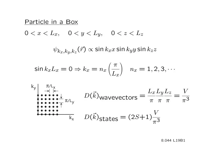
Particle in a Box 0 < x < L x , 0 < y < L y , 0 < z - PowerPoint PPT Presentation

Particle in a Box 0 < x < L x , 0 < y < L y , 0 < z < L z ψ k x ,k y ,k z ( r r ) ∝ sin k x x sin k y y sin k z z π � � sin k x L x = 0 ⇒ k x = n x n x = 1 , 2 , 3 , · · · L x � � π ��� L x L y L z V D ( r k )wavevectors = π π π = π 3 π ��� V D ( r k )states = (2 S +1) π 3 � � 8.044 L19B1

r ) ∝ exp[ ir Plane Wave ψ r ( r r ] k · r k Periodic Boundary Conditions ψ r ( r r + m x L x x ˆ + m y L y y ˆ+ m z L z z ˆ) = ψ r ( r r ) k k 2 π � � ik x ( x + m x L x ) ik x x ⇒ k x = e = n x n x = ± 1 , ± 2 , ± 3 , · · · e L x � � L x L y L z V D ( r k )wavevectors = 2 π 2 π 2 π = � π ��� (2 π ) 3 � π ��� V D ( r k )states = (2 S +1) � � (2 π ) 3 8.044 L19B 2

The # of wavevectors with | - k ' | < k is the same in both cases. 1 4 4 V V πk 3 πk 3 #wavevectors( k ) = 8 = π 3 (2 π ) 3 3 3 n 2 k 2 2 m √ For free particles; E = → k ( E ) = E n 2 2 m 3 / 2 4 V V 2 m πk ( E ) 3 E 3 / 2 #wv( E ) = = (2 π ) 3 6 π 2 n 2 3 3 / 2 d V 2 m E 1 / 2 D wv( E ) = #wv( E ) = 4 π 2 n 2 dE 8.044 L19B3

For free particles � 3 / 2 V 2 m � E 1 / 2 D states( E ) = (2 S + 1) 4 π 2 n 2 �� ε � ε 8.044 L19B4

Fermions: Non-interacting, free, spin 1/2, T = 0 k z D( ε ) k F k y ε F ε k x Fermi sea Fermi wave vector k F Fermi energy E F = n 2 k F 2 / 2 m Fermi surface 8.044 L19B5

N = 2 × D wavevectors( k ) × 4 3 = 8 V 3 πk F π k F 3 (2 π ) 3 3 � 1 / 3 3 π 2 ( N/V ) ∝ ( N/V ) 1 / 3 � k F = ⎞ 2 / 3 n 2 k 2 n 2 3 π 2 N ⎛ ∝ ( N/V ) 2 / 3 F E F = = ⎝ ⎠ 2 m 2 m V 8.044 L19B6

D ( � ) = a � 1 / 2 � � F 3 / 2 2 N = D ( � ) d� = 3 a � F 0 � � F 5 / 2 2 3 ∝ N ( N/V ) 2 / 3 U = �D ( � ) d� = 5 a � = 5 N� F F 0 8.044 L19B7

Consequences: Motion at T = 0 ¯ hP hP h P = ¯ p F = ¯ v F = p k P k F k F m Copper, one valence electron beyond a filled d shell N/V = 8 . 45 × 10 22 atoms-cm − 3 k F = 1 . 36 × 10 8 cm − 1 v F = 1 . 57 × 10 8 cm-s − 1 p F = 1 . 43 × 10 − 19 g-cm-s − 1 E F /k B = 81 , 000 K 8.044 L 19 B 8

Consequences: P ( T = 0) 3 E F ∝ ( N/V ) 2 / 3 U = 5 NE F � � � � ∂U ∂E F = − 3 2 P = − = ( N/V ) E F 5 N 5 ∂V N,S ∂V N ' N EF − 2 3 V ∝ ( N/V ) 5 / 3 � � ∂P = − 5 ( P/V ) at T = 0 3 ∂V N,T 8.044 L19B9

1 �V 3 1 3 1 � � K T = − = = V �P N,T 5 P 2 ( N/V ) E F For potassium E F = 2 . 46 × 10 4 K = 3 . 39 × 10 − 12 ergs ( N/V ) conduction = 1 . 40 × 10 22 cm − 3 1 . 5 K T = 1 . 40 × 10 22 × 3 . 39 × 10 − 12 = 31 . 6 × 10 − 12 cm -ergs 3 − 1 The measued value is 31 × 10 − 12 ! 8.044 L 19 B 10

Magnetic Susceptibility ε P H = Hz ˆ ε F E k, � = E ( k ) + µ e H E k, � = E ( k ) − µ e H µ e H D ( ε ) D ( ε ) 8.044 L 19 B 11

    2 + µ e H D ( � F ) 2 − µ e H D ( � F )  N  −  N N � − N � =  2 2 2 HD ( � F ) ≡ χH = µ e HD ( � F ) M = µ � e 2 D ( � F ) χ = µ e This expression holds as long as kT « � F , so χ is temperature independent in this region. This is not Curie law behavior. It is called Pauli paramagnetism. 8.044 L 19 B1 2

Temperature Dependence of < n P > k,m s < n P > = f ( E ) only, as in the Canonical Ensemble k,m s <n> ~ kT 1 T=0 T << ε F /k B ε F ε 8.044 L 19 B 13

Estimate C V Classical Quantum # electrons N N ∼ N × kT # electrons influenced N � F 3 ∆ � 2 kT ∼ kT ∼ N ( kT ) 2 3 ∆ U 2 NkT � F 3 ∼ 2 Nk kT C V 2 Nk � F Exact result: C V = π 2 2 Nk kT � F 8.044 L19B14

� ∞ N = < n ( �, µ ( T ) , T ) > D ( � ) d� 0 This expression implicitly determines µ = µ ( T ). � ∞ U = < n ( �, µ ( T ) , T ) > � D ( � ) d� 0 To determine C V from this expression one must take into account the temperature dependence of µ in addition to the explicit dependence of < n > on T . 8.044 L19B15

��� ���� � ��� ����� ε � �� � ε � ε < n > − 1 / 2 = − < n > − 1 / 2 [ ] [ ] [ ] [ ] at E = µ + δ at E = µ − δ 8.044 L19B16

�� ε � � ε µ ε � Because D ( � ) is an increasing function of � , µ must decrease with increasing temperature. 8.044 L19B17

Elementary Excitations Excitations out of the ground state in interacting many-body systems. For a 3D Coulomb gas of electrons Plasma oscillations (plasmons) ε ��� Collective modes: H.O.s Quasi-particles n 2 k 2 (‘dressed’ electrons) = 2 m ∗ � 8.044 L19B18

Other collective modes Phonons, lattice vibrations in solids Spin waves, in Ferromagnets Ripplons, waves on surfaces Other quasi-particles Polarons, (electron+lattice distortion) in ionic materials 8.044 L19B19

Some possible electronic densities of states in solids �� ε � �� ε � ����� ��������� ε � ε ε ���� �� ε � �� ε � ����������������������� ������������������� ε � ε ε ε � ������ 8.044 L19B20

Finding µ ( T ) in an intrinsic semiconductor ��� �� ε � � � ε ε � µ ε � Assume the energy gap is � k B T . 8.044 L19B21

� �� �� �� �� �� � � � � � � Comparison of 1 / ( e x + 1) with e − x when x > 0 and x 1 − e when x < 0. 8.044 L19B21a

− ( E − µ ) /k B T − ( E G − µ ) /k B T − ( E − E G ) /k B T < n e > → e = e e � 3 / 2 � 2 m e V ( E − E G ) 1 / 2 D states ,e ( E ) = 2 π 2 n 2 � ∞ N e = < n e > D ( E ) dE E G � 3 / 2 − ( E G − µ ) /k B T V 2 m e � ∞ √ � δ e − δ/k B T dδ = 2 π 2 e n 2 0 � 3 / 2 V 2 m e k B T � − ( E G − µ ) /k B T = e π n 2 4 8.044 L19B22

− ( µ − E ) /k B T < n h > = 1 − < n e > → e � 3 / 2 2 m h V � ( − E ) 1 / 2 D states ,h ( E ) = 2 π 2 n 2 � 0 N h = < n h > D ( E ) dE −∞ � 3 / 2 � ∞ √ V 2 m h � − µ/k B T δ e − δ/k B T dδ = 2 π 2 e n 2 0 � 3 / 2 V 2 m h k B T � − µ/k B T = e π n 2 4 8.044 L19B23

N h = N e 3 / 2 − µ/k B T 3 / 2 − ( � G − µ ) /k B T m e = m e e h ( m h /m e ) 3 / 2 = e − � G /k B T e 2 µ/k B T (3 / 2) k B T ln( m h /m e ) = − � G + 2 µ µ = � G / 2 − (3 / 4) k B T ln( m e /m h ) 8.044 L19B24

MIT OpenCourseWare http://ocw.mit.edu 8.044 Statistical Physics I Spring 2013 For information about citing these materials or our Terms of Use, visit: http://ocw.mit.edu/terms.