Part III: The Nuclear Many-Body Problem To understand the properties - PowerPoint PPT Presentation

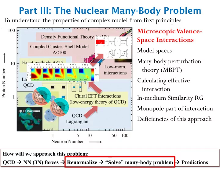
Part III: The Nuclear Many-Body Problem To understand the properties of complex nuclei from first principles Microscopic Valence- Space Interactions Model spaces Many-body perturbation theory (MBPT) Calculating effective interaction In-medium Similarity RG Monopole part of interaction Deficiencies of this approach How will we approach this problem: QCD à à NN (3N) forces à à Renormalize à à “Solve” many-body problem à à Predictions

The Nuclear Many-Body Problem Nucleus strongly interacting many-body system – how to solve A -body problem? H ψ n = E n ψ n Quasi-exact solutions only in light nuclei (GFMC, NCSM…) Large scale : controlled approximations to full Schrödinger Equation Valence space : diagonalize exactly with reduced number of degrees of freedom Medium-mass Medium-mass Large scale Valence space Limited range: All nuclei near closed-shell cores Closed shell ±1 Even-even All properties: Ground states Limited properties: Excited states Ground states only Some excited state EW transitions Coupled Cluster Coupled Cluster In-Medium SRG In-Medium SRG Green’s Function Perturbation Theory

From Momentum Space to HO Basis To this point interaction matrix elements in momentum space, partial waves h kK, lL | V | k 0 K, l 0 L i α To go to finite nuclei begin from Hamiltonian H ψ n = ( T + V ) ψ n = E n ψ n Assume many particles in the nucleus generate a mean field U : U a one-body potential simple to solve (typically Harmonic Oscillator ) H = H 0 + H 1 ; H 0 = T + U ; H 1 = V − U So transform from momentum space to Harmonic Oscillator Basis ⇣ p Z ⌘ ⇣p ⌘ k 2 d k K 2 d K R nl | nl, NL ; α i = 2 α k R NL 1 / 2 α K | kl, KL ; α i One more (ugly) transformation from center-of-mass to lab frame: ! h ab ; JT | V | cd ; JT i

Valence-Space Ideas Begin with degenerate HO levels 112 0 h , 1 f , 2 p 70 0 g ,1 d ,2 s 40 0 f ,1 p 20 0 d ,1 s 8 0 p 2 0 s h ab ; JT | V | cd ; JT i Physics of V breaks HO degeneracy Problem : Can’t solve Schrodinger equation in full Hilbert space

Valence-Space Ideas Nuclei understood as many-body system starting from closed shell, add nucleons Unperturbed Removes degeneracy in HO spectrum valence space only 112 112 0 h , 1 f , 2 p 0 h , 1 f , 2 p 70 70 0 g ,1 d ,2 s 0 g ,1 d ,2 s Active nucleons occupy 40 40 0 f ,1 p 0 f ,1 p valence space 20 0d 3/2 20 0 d ,1 s 1s 1/2 0d 5/2 “sd”-valence space 8 8 0 p 0 p 2 Assume filled core 2 0 s 0 s

Valence-Space Ideas Nuclei understood as many-body system starting from closed shell, add nucleons Valence-space Hamiltonian derived from nuclear forces: Single-particle energies X ε i a † H v . s . = i a i + V v . s . Interaction matrix elements i 112 0 h , 1 f , 2 p 70 0 g ,1 d ,2 s 40 c 0 f ,1 p d 20 0d 3/2 “sd” 1s 1/2 V valence space 0d 5/2 a b 8 Active nucleons occupy Inert 0 p valence space 2 0 s

Valence-Space Philosophy Nuclei understood as many-body system starting from closed shell, add nucleons Valence-space Hamiltonian derived from nuclear forces: Single-particle energies X ε i eff a † H e ff = i a i + V e ff Interaction matrix elements i H ψ n = E n ψ n → PH e ff P ψ i = E i P ψ i 112 0 h , 1 f , 2 p Effective valence space Hamiltonian : 70 0 g ,1 d ,2 s Sum all excitations outside valence space 40 c c 0 f ,1 p d d 20 V eff 0d 3/2 “sd” 1s 1/2 V valence space 0d 5/2 a a b b 8 Inert 0 p Decouple valence space from excitations 2 0 s

Perturbative Approach 1) Effective Hamiltonian: sum excitations outside valence space 2) Self-consistent single-particle energies x c c a a a d d V low-k d N max k ε eff 112 + . . . 0 h , 1 f , 2 p = + a a V a a a b b b 70 0 g ,1 d ,2 s c c c d d d 40 0 f ,1 p V eff ˆ = + Q 20 V 0d 3/2 a a 1s 1/2 a b b b 0d 5/2 c c d d 8 0 p + + . . . + + a a 2 b b 0 s

Perturbative Approach 1) Effective Hamiltonian: sum excitations outside valence space to MBPT(3) 2) Self-consistent single-particle energies c c c d d d V eff ˆ = + Q V a a a b b b c c d d + + . . . + + a a b b

Perturbative Approach 1) Effective Hamiltonian: sum excitations outside valence space to MBPT(3) 2) Self-consistent single-particle energies 3) Harmonic-oscillator basis of 13-15 major shells: converged! -2 Single-Particle Energy (MeV) 4 Neutron Proton f 5/2 -4 f 5/2 2 -6 p 1/2 p 1/2 0 -8 -2 f 7/2 f 7/2 -10 p 3/2 p 3/2 -4 -12 2 4 6 8 10 12 14 16 18 2 4 6 8 10 12 14 16 18 _ � _ � Nh Nh

Perturbative Approach 1) Effective Hamiltonian: sum excitations outside valence space to MBPT(3) 2) Self-consistent single-particle energies 3) Harmonic-oscillator basis of 13-15 major shells: converged! -10.5 -18.5 -76 Ground-State Energy (MeV) -77 18 O -11 -19 Energy (MeV) -78 42 Ca 48 Ca V low k (1st) -11.5 -19.5 V low k (2nd) -79 V low k (3rd) 1st order -80 -12 2nd order -20 3rd order -81 -12.5 -20.5 -82 4 6 8 10 12 14 2 4 6 8 10 12 14 16 18 2 4 6 8 10 12 14 16 18 _ � _ � Major Shells Nh Nh

Aside: G-matrix Renormalization Standard method for softening interaction in nuclear structure for decades: Infinite summation of ladder diagrams Need two model spaces: 1) M space in which we will want to calculate (excitations allowed in M) 2) Large space Q in which particle excitations are allowed To avoid double counting, can’t overlap – matrix elements depend on M

Aside: G-matrix Renormalization Standard method for softening interaction in nuclear structure for decades: Q X G ijkl ( ω ) = V ijkl + G mnkl ( ω ) V ijmn ω − ε m − ε n mn ∈ Q Iterative procedure Dependence on arbitrary starting energy!

G-matrix Renormalization Standard method for softening interaction in nuclear structure for decades: Q X G ijkl ( ω ) = V ijkl + G mnkl ( ω ) V ijmn ω − ε m − ε n What happens mn ∈ Q as we keep increasing M?

G-matrix Renormalization Results of G-matrix renormalization vs. SRG AV1 V18 SR SRG N 3 LO LO SRG SR SR SRG+ G+ SRG+ SR G+ G-m G-mat G-m G-mat G-mat G-m G-m G-mat Removes some diagonal high-momentum components Still large low-to-high coupling in both interactions No indication of universality Clear difference compared with SRG-evolved interactions!

Perturbative Approach 1) Effective Hamiltonian: sum excitations outside valence space to MBPT(3) 2) Self-consistent single-particle energies 3) Harmonic-oscillator basis of 13-15 major shells: converged! -11.6 rd order nd order 3 2 18 O -11.8 Energy (MeV) -12 -12.2 V low k -12.4 G-matrix -12.6 4 6 8 10 12 14 2 4 6 8 10 12 14 Major Shells Major Shells Compare vs G-matrix (no sign of convergence) Clear benefit of low-momentum interactions!

Perturbative Approach 1) Effective Hamiltonian: sum excitations outside valence space to MBPT(3) 2) Self-consistent single-particle energies 3) Harmonic-oscillator basis of 13-15 major shells 4) Nuclear forces from chiral EFT 5) Requires extended valence spaces 50 50 Treat higher orbits nonperturbatively 0 g 9/2 0g 9/2 0f 5/2 0f 5/2 1 p 1/2 1p 1/2 1p 3/2 1p 3/2 28 28 0f 7/2 0f 7/2 20 20 0 d 3/2 0d 3/2 1 s 1/2 1s 1/2 0 d 5/2 0d 5/2 16 O 8 8 0p 3/2 0p 3/2 0p 1/2 0p 1/2

Limits of Nuclear Existence: Oxygen Anomaly Where is the nuclear dripline? Limits defined as last isotope with positive neutron separation energy - Nucleons “drip” out of nucleus Neutron dripline experimentally established to Z=8 (Oxygen)

Limits of Nuclear Existence: Oxygen Anomaly Where is the nuclear dripline? Limits defined as last isotope with positive neutron separation energy - Nucleons “drip” out of nucleus Neutron dripline experimentally established to Z=8 (Oxygen) Regular dripline trend… except oxygen Adding one proton binds 6 additional neutrons

Limits of Nuclear Existence: Oxygen Anomaly Where is the nuclear dripline? Limits defined as last isotope with positive neutron separation energy - Nucleons “drip” out of nucleus Neutron dripline experimentally established to Z=8 (Oxygen) Prediction with NN forces Microscopic picture: NN-forces too attractive Incorrect prediction of dripline

Monopole Part of Valence-Space Interactions Microscopic MBPT – effective interaction in chosen model space Works near closed shells: deteriorates beyond this Deficiencies improved adjusting particular two-body matrix elements Monopoles: J (2 J + 1) V JT P V T abab ab = Angular average of interaction P J (2 J + 1) Determines interaction of orbit a with b: evolution of orbital energies 1 Δ ε a = V ab n b 0.5 T=1 0 Microscopic low-momentum interactions V(ab;T) [MeV] -0.5 Phenomenological USD interactions -1 V low k -1.5 Clear shifts in low-lying orbitals : USDa -2 USDb - T=1 repulsive shift -2.5 -3 -3.5 d5d5 d5d3 d5s1 d3d3 d3s1 s1s1

Physics in Oxygen Isotopes Calculate evolution of sd -orbital energies from interactions 20 - 16 O - 22 O - 24 O - 28 O - 16 O - 22 O - 24 O - 28 O 0d 3/2 1s 1/2 0d 5/2 - 16 O 8 0p 3/2 Fit to experiment 0p 1/2 Microscopic NN Theories Phenomenological Models d 3/2 orbit bound to 28 O d 3/2 orbit unbound