Page 1 1 Review: Projection Taxonomy Review: Midpoint Algorithm - - PDF document

SLIDE 1

1

Page 1

University of British Columbia CPSC 314 Computer Graphics May-June 2005 Tamara Munzner http://www.ugrad.cs.ubc.ca/~cs314/Vmay2005

Lighting/Shading I, II, III Week 3, Tue May 24

• News

P1 demos if you missed them 3:30-4:30 today

• Homework 2 Clarification
• ff-by-one problem in Q4-6

Q4 should refer to result of Q1 Q5 should refer to result of Q2 Q6 should refer to result of Q3

acronym confusion

Q1 uses W2C, whereas notes say W2V world to camera/view/eye Q2 uses C2P, whereas notes say V2C, C2N Q3 uses N2V, whereas notes say N2D normalized device to viewport/device

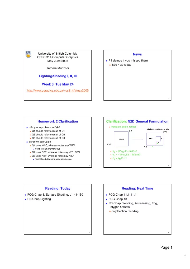
• Clarification: N2D General Formulation

(-1,-1) (1,1) (1,1) (0,0) (0,0) (w,h) (w,h) NDCS NDCS DCS DCS

glViewport(c,d,a,b);

a b c d

xD = (a*xN)/2 + (a/2)+c yD = - ((b*yN)/2 + (b/2)+d) zD = zN/2 + 1 translate, scale, reflect

• Reading: Today

FCG Chap 8, Surface Shading, p 141-150 RB Chap Lighting

• Reading: Next Time

FCG Chap 11.1-11.4 FCG Chap 13 RB Chap Blending, Antialiasing, Fog,

Polygon Offsets

• nly Section Blending

SLIDE 2

2

Page 2

• Review: Projection Taxonomy

planar planar projections projections perspective: perspective: 1,2,3 1,2,3-point point parallel parallel

• blique
• blique
• rthographic
• rthographic

cabinet cabinet cavalier cavalier top, top, front, front, side side axonometric: axonometric: isometric isometric dimetric dimetric trimetric trimetric

http://ceprofs.tamu.edu/tkramer/ENGR%20111/5.1/20

• Review: Midpoint Algorithm

moving horizontally along x direction

draw at current y value, or move up vertically to y+1? check if midpoint between two possible pixel centers

above or below line

candidates

top pixel: (x+1,y+1) bottom pixel: (x+1, y)

midpoint: (x+1, y+.5) check if midpoint above or below line

below: top pixel above: bottom pixel

key idea behind Bresenham

[demo]

• P

Review: Flood Fill

simple algorithm draw edges of polygon use flood-fill to draw interior

• Review: Scanline Algorithms

scanline: a line of pixels in an image set pixels inside polygon boundary along

horizontal lines one pixel apart vertically

1 2 3 4 5=0 P

• Review: General Polygon Rasterization

idea: use a parity test

for each scanline edgeCnt = 0; for each pixel on scanline (l to r) if (oldpixel->newpixel crosses edge) edgeCnt ++; // draw the pixel if edgeCnt odd if (edgeCnt % 2) setPixel(pixel);

Review: Making It Fast: Bounding Box

smaller set of candidate pixels loop over xmin, xmax and ymin,ymax

instead of all x, all y

SLIDE 3

3

Page 3

• Review: Bilinear Interpolation

interpolate quantity along L and R edges,

as a function of y

then interpolate quantity as a function of x

y y P(x,y) P(x,y) P P1 P P2 P P3 P PL P PR

• Review: Barycentric Coordinates

weighted combination of vertices smooth mixing speedup

compute once per triangle

1

P

3

P

2

P P

( (α,β,γ α,β,γ α,β,γ α,β,γ α,β,γ α,β,γ α,β,γ α,β,γ) = ) = (1,0,0) (1,0,0) ( (α,β,γ α,β,γ α,β,γ α,β,γ α,β,γ α,β,γ α,β,γ α,β,γ) = ) = (0,1,0) (0,1,0) ( (α,β,γ α,β,γ α,β,γ α,β,γ α,β,γ α,β,γ α,β,γ α,β,γ) = ) = (0,0,1) (0,0,1)

5 . = β 1 = β = β

3 2 1

P P P P ⋅ + ⋅ + ⋅ = γ β α 1 , , 1 ≤ ≤ = + + γ β α γ β α

“ “convex combination convex combination

• f points”
• f points”

for points inside triangle

• Review: Deriving Barycentric Coordinates

non-orthogonal

coordinate system

P3 is origin, P2-P3, P1-

P3 are basis vectors

from bilinear

interpolation of point P

• n scanline

1

P

3

P

2

P P

(1,0,0) (1,0,0) (0,1,0) (0,1,0) (0,0,1) (0,0,1)

P P2 P P3 P P1 P PL P PR P P d d

2 2

: d : d

1 1

• Correction/Review: Deriving Barycentric

Coordinates

2D triangle area

3

P

A

1

P

3

P

2

P P

( (α,β,γ α,β,γ α,β,γ α,β,γ α,β,γ α,β,γ α,β,γ α,β,γ) = ) = (1,0,0) (1,0,0) ( (α,β,γ α,β,γ α,β,γ α,β,γ α,β,γ α,β,γ α,β,γ α,β,γ) = ) = (0,1,0) (0,1,0) ( (α,β,γ α,β,γ α,β,γ α,β,γ α,β,γ α,β,γ α,β,γ α,β,γ) = ) = (0,0,1) (0,0,1)

A A A A A A

P P P

/ / /

1 2 3

= = = γ β α

2

P

A

1

P

A

1 2 3

P P P

A A A A + + + =

AP3 AP1

• Review: Simple Model of Color

simple model based on RGB triples component-wise multiplication of colors

(a0,a1,a2) * (b0,b1,b2) = (a0*b0, a1*b1, a2*b2) why does this work?

• Review: Trichromacy and Metamers

three types of cones color is combination

• f cone stimuli

metamer: identically

perceived color caused by very different spectra

SLIDE 4

4

Page 4

• Review: Color Constancy
• Clarification/Review: Stroop Effect

blue green purple red

• range

say what color the text is as fast as possible interplay between cognition and perception

• Review: Measured vs. CIE Color Spaces
• measured basis
• monochromatic lights
• physical observations
• negative lobes

transformed basis “imaginary” lights all positive, unit area Y is luminance

• Review: Device Color Gamuts

compare gamuts on CIE chromaticity diagram gamut mapping

• Review: RGB Color Space

define colors with (r, g, b)

amounts of red, green, and blue

used by OpenGL

RGB color cube sits within

CIE color space

subset of perceivable colors

• Review: Additive vs. Subtractive Colors

additive: light monitors, LCDs RGB model subtractive: pigment printers CMY model

• −
• =
• B

G R Y M C 1 1 1

SLIDE 5

5

Page 5

• Review: HSV Color Space

hue: dominant wavelength, “color” saturation: how far from grey value/brightness: how far from

black/white

cannot convert to RGB with matrix

alone

• Review: YIQ Color Space

color model used for color TV Y is luminance (same as CIE) I & Q are color (not same I as HSI!) using Y backwards compatible for B/W TVs conversion from RGB is linear

green is much lighter than red, and red lighter

than blue

• −

− − =

• B

G R Q I Y 31 . 52 . 21 . 32 . 28 . 60 . 11 . 59 . 30 .

Q I

• Review: Monitors

monitors have nonlinear response to input characterize by gamma

displayedIntensity = aγ

γ γ γ (maxIntensity)

gamma correction displayedIntensity = (maxIntensity)

= a (maxIntensity)

γ γ

• /

1 a

• Lighting I
• Goal

model interaction of light with matter in a way that appears realistic and is fast

phenomenological reflection models

ignore real physics, approximate the look simple, non-physical Phong, Blinn-Phong

physically based reflection models

simulate physics BRDFs: Bidirectional Reflection Distribution

Functions

• Photorealistic Illumination

[ [electricimage.com electricimage.com] ]

SLIDE 6

6

Page 6

• Photorealistic Illumination

[ [electricimage.com electricimage.com] ]

• Fast Local Illumination
• Illumination

transport of energy from light sources to

surfaces & points

• includes direct and indirect illumination

Images by Henrik Wann Jensen

• Components of Illumination

two components: light sources and surface properties light sources (or emitters)

• spectrum of emittance (i.e., color of the light)
• geometric attributes

position direction shape

directional attenuation polarization

• Components of Illumination

surface properties

• reflectance spectrum (i.e., color of the surface)

subsurface reflectance geometric attributes position

• rientation

micro-structure

• heat/light source

thermometer/eye reflective objects energy packets

Illumination as Radiative Transfer

radiative heat transfer approximation substitute light for heat light as packets of energy (photons)

particles not waves

model light transport as packet flow

SLIDE 7

7

Page 7

• light waves

single slit new wavefront light particles single slit bent ray?!

Light Transport Assumptions

• geometrical optics (light is photons not waves)

no diffraction no polarization (some sunglasses) light of all orientations gets through no interference (packets don’t interact) which visual effects does this preclude?

• Light Transport Assumptions II

color approximated by discrete wavelengths quantized approx of dispersion (rainbows) quantized approx of fluorescence (cycling

vests)

no propagation media (surfaces in vacuum) no atmospheric scattering (fog, clouds)

some tricks to simulate explicitly

no refraction (mirages) light travels in straight line no gravity lenses

superposition (lights can be added)

• Light Sources and Materials

appearance depends on light sources, locations, properties material (surface) properties viewer position local illumination compute at material, from light to viewer global illumination (later in course) ray tracing: from viewer into scene radiosity: between surface patches

• Illumination in the Pipeline

local illumination

• nly models light arriving directly from light

source

no interreflections and shadows

can be added through tricks, multiple

rendering passes

light sources simple shapes materials simple, non-physical reflection models

• Light Sources

types of light sources

• glLightfv(GL_LIGHT0,GL_POSITION,light[])

directional/parallel lights

real-life example: sun infinitely far source: homogeneous coord w=0

point lights

same intensity in all directions

spot lights

limited set of directions: point+direction+cutoff angle

• z

y x

• 1

z y x

• Light Sources

area lights light sources with a finite area more realistic model of many light sources not available with projective rendering pipeline,

(i.e., not available with OpenGL)

SLIDE 8

8

Page 8

• Light Sources

ambient lights no identifiable source or direction hack for replacing true global illumination

(light bouncing off from other objects)

• Ambient Light Sources

scene lit only with an ambient light source Light Position Not Important Viewer Position Not Important Surface Angle Not Important

• Directional Light Sources

scene lit with directional and ambient light Light Position Not Important Viewer Position Not Important Surface Angle Important

• Point Light Sources

scene lit with ambient and point light source Light Position Important Viewer Position Important Surface Angle Important

• Light Sources

geometry: positions and directions standard: world coordinate system

effect: lights fixed wrt world geometry demo:

http://www.xmission.com/~nate/tutors.html

alternative: camera coordinate system

effect: lights attached to camera (car headlights)

points and directions undergo normal

model/view transformation

illumination calculations: camera coords

• Types of Reflection

specular (a.k.a. mirror or regular) reflection causes

light to propagate without scattering.

diffuse reflection sends light in all directions with

equal energy.

mixed reflection is a weighted

combination of specular and diffuse.

SLIDE 9

9

Page 9

• Types of Reflection

retro-reflection occurs when incident energy

reflects in directions close to the incident direction, for a wide range of incident directions.

gloss is the property of a material surface

that involves mixed reflection and is responsible for the mirror like appearance of rough surfaces.

• Reflectance Distribution Model

most surfaces exhibit complex reflectances

vary with incident and reflected directions. model with combination

+ + = specular + glossy + diffuse = reflectance distribution

• Surface Roughness

at a microscopic scale, all

real surfaces are rough

cast shadows on

themselves

“mask” reflected light: shadow shadow Masked Light

• Surface Roughness

notice another effect of roughness:

each “microfacet” is treated as a perfect mirror. incident light reflected in different directions by

different facets.

end result is mixed reflectance. smoother surfaces are more specular or glossy. random distribution of facet normals results in diffuse

reflectance.

• Physics of Diffuse Reflection

ideal diffuse reflection very rough surface at the microscopic level

real-world example: chalk

microscopic variations mean incoming ray of

light equally likely to be reflected in any direction over the hemisphere

what does the reflected intensity depend on?

• Lambert’s Cosine Law

ideal diffuse surface reflection

the energy reflected by a small portion of a surface from a light source in a given direction is proportional to the cosine

• f the angle between that direction and the surface normal

reflected intensity independent of viewing direction depends on surface orientation wrt light

• ften called Lambertian surfaces

SLIDE 10

10

Page 10

• Lambert’s Law

intuitively: cross-sectional area of the “beam” intersecting an element

• f surface area is smaller for greater

angles with the normal.

• Computing Diffuse Reflection

depends on angle of incidence: angle between surface

normal and incoming light

• Idiffuse = kd Ilight cos θ

in practice use vector arithmetic

• Idiffuse = kd Ilight (n • l)

always normalize vectors used in lighting

• n, l should be unit vectors

scalar (B/W intensity) or 3-tuple or 4-tuple (color)

• kd: diffuse coefficient, surface color
• Ilight: incoming light intensity
• Idiffuse: outgoing light intensity (for diffuse reflection)

n l θ

• Diffuse Lighting Examples

Lambertian sphere from several lighting

angles:

need only consider angles from 0°to 90° why? demo: Brown exploratory on reflection

• http://www.cs.brown.edu/exploratories/freeSoftware/repository/edu/brown/cs/ex

ploratories/applets/reflection2D/reflection_2d_java_browser.html

• Lighting II
• diffuse

diffuse plus specular

Specular Reflection

shiny surfaces exhibit specular reflection

polished metal glossy car finish

specular highlight

bright spot from light shining on a specular surface

view dependent

highlight position is function of the viewer’s position

• Physics of Specular Reflection

at the microscopic level a specular reflecting

surface is very smooth

thus rays of light are likely to bounce off the

microgeometry in a mirror-like fashion

the smoother the surface, the closer it

becomes to a perfect mirror

SLIDE 11

11

Page 11

• Optics of Reflection

reflection follows Snell’s Law: incoming ray and reflected ray lie in a plane

with the surface normal

angle the reflected ray forms with surface

normal equals angle formed by incoming ray and surface normal θ(l)ight = θ(r)eflection

• Non-Ideal Specular Reflectance

Snell’s law applies to perfect mirror-like surfaces,

but aside from mirrors (and chrome) few surfaces exhibit perfect specularity

how can we capture the “softer” reflections of

surface that are glossy, not mirror-like?

• ne option: model the microgeometry of the

surface and explicitly bounce rays off of it

• r…
• Empirical Approximation

we expect most reflected light to travel in

direction predicted by Snell’s Law

but because of microscopic surface

variations, some light may be reflected in a direction slightly off the ideal reflected ray

as angle from ideal reflected ray increases,

we expect less light to be reflected

• Empirical Approximation
• angular falloff

how might we model this falloff?

• Phong Lighting

most common lighting model in computer graphics

• (Phong Bui-Tuong, 1975)

nshiny : purely empirical

constant, varies rate of falloff

ks: specular coefficient,

highlight color

no physical basis, works

• k in practice

v

Ispecular = ksIlight(cosφ)nshiny

• Phong Lighting: The nshiny Term

Phong reflectance term drops off with divergence of viewing

angle from ideal reflected ray

what does this term control, visually?

Viewing angle – reflected angle

SLIDE 12

12

Page 12

• Phong Examples

varying l varying nshiny

• Calculating Phong Lighting

compute cosine term of Phong lighting with vectors

v: unit vector towards viewer/eye r: ideal reflectance direction (unit vector) ks: specular component

highlight color

• Ilight: incoming light intensity

how to efficiently calculate r ?

v

Ispecular = ksIlight(v•r)nshiny

• Calculating R Vector

P = N cos θ = projection of L onto N

L P N

θ

• Calculating R Vector

P = N cos θ = projection of L onto N P = N ( N · L )

L P N

θ

• Calculating R Vector

P = N cos θ |L| |N| projection of L onto N P = N cos θ L, N are unit length P = N ( N · L )

L P N

θ

• Calculating R Vector

P = N cos θ |L| |N| projection of L onto N P = N cos θ L, N are unit length P = N ( N · L ) 2 P = R + L 2 P – L = R 2 (N ( N · L )) - L = R

L P P R L N

θ

SLIDE 13

13

Page 13

• Phong Lighting Model

combine ambient, diffuse, specular components commonly called Phong lighting

• nce per light
• nce per color component

Itotal = ksIambient + Ii(

i=1 # lights

• kd(n•li) + ks(v•ri)nshiny )
• Phong Lighting: Intensity Plots
• Blinn-Phong Model

variation with better physical interpretation

Jim Blinn, 1977

h: halfway vector

h must also be explicitly normalized: h / |h| highlight occurs when h near n

l l n n v v h h Iout(x) = ks(h•n)nshiny • Iin(x);with h = (l + v)/2

• Light Source Falloff

quadratic falloff brightness of objects depends on power per

unit area that hits the object

the power per unit area for a point or spot light

decreases quadratically with distance

Area Area 4 4π πr r2 Area Area 4 4π π(2 (2r) r)2

• Light Source Falloff

non-quadratic falloff many systems allow for other falloffs allows for faking effect of area light sources OpenGL / graphics hardware

Io: intensity of light source x: object point r: distance of light from x

2

1 ) ( I c br ar Iin ⋅ + + = x

• Lighting Review

lighting models ambient

normals don’t matter

Lambert/diffuse

angle between surface normal and light

Phong/specular

surface normal, light, and viewpoint

SLIDE 14

14

Page 14

• Lighting in OpenGL

light source: amount of RGB light emitted

value represents percentage of full intensity

e.g., (1.0,0.5,0.5)

every light source emits ambient, diffuse, and specular

light

materials: amount of RGB light reflected

value represents percentage reflected

e.g., (0.0,1.0,0.5)

interaction: multiply components

red light (1,0,0) x green surface (0,1,0) = black (0,0,0)

• Lighting in OpenGL

glLightfv(GL_LIGHT0, GL_AMBIENT, amb_light_rgba ); glLightfv(GL_LIGHT0, GL_DIFFUSE, dif_light_rgba ); glLightfv(GL_LIGHT0, GL_SPECULAR, spec_light_rgba ); glLightfv(GL_LIGHT0, GL_POSITION, position); glEnable(GL_LIGHT0); glMaterialfv( GL_FRONT, GL_AMBIENT, ambient_rgba ); glMaterialfv( GL_FRONT, GL_DIFFUSE, diffuse_rgba ); glMaterialfv( GL_FRONT, GL_SPECULAR, specular_rgba ); glMaterialfv( GL_FRONT, GL_SHININESS, n ); warning: glMaterial is expensive and tricky

use cheap and simple glColor when possible see OpenGL Pitfall #14 from Kilgard’s list

http://www.opengl.org/resources/features/KilgardTechniques/oglpitfall/

• Shading
• Lighting vs. Shading

lighting process of computing the luminous intensity

(i.e., outgoing light) at a particular 3-D point, usually on a surface

shading the process of assigning colors to pixels (why the distinction?)

• Applying Illumination

we now have an illumination model for a point

• n a surface

if surface defined as mesh of polygonal facets,

which points should we use?

fairly expensive calculation several possible answers, each with different

implications for visual quality of result

• Applying Illumination

polygonal/triangular models each facet has a constant surface normal if light is directional, diffuse reflectance is

constant across the facet.

why?

SLIDE 15

15

Page 15

• Flat Shading

simplest approach calculates illumination at a

single point for each polygon

• bviously inaccurate for smooth surfaces
• Flat Shading Approximations

if an object really is faceted,

is this accurate?

no! for point sources, the

direction to light varies across the facet

for specular reflectance,

direction to eye varies across the facet

• Improving Flat Shading

what if evaluate Phong lighting model at each pixel

• f the polygon?

better, but result still clearly faceted

for smoother-looking surfaces

we introduce vertex normals at each vertex

usually different from facet normal used only for shading think of as a better approximation of the real surface

that the polygons approximate

• Vertex Normals

vertex normals may be provided with the model computed from first principles approximated by

averaging the normals

• f the facets that

share the vertex

• Gouraud Shading

most common approach, and what OpenGL does

perform Phong lighting at the vertices linearly interpolate the resulting colors over faces along edges along scanlines

C1 C2 C3 edge: mix of c1, c2 edge: mix of c1, c3 interior: mix of c1, c2, c3

does this eliminate the facets?

• Gouraud Shading Artifacts
• ften appears dull, chalky

lacks accurate specular component if included, will be averaged over entire

polygon

C1 C2 C3 this interior shading missed! C1 C2 C3 this vertex shading spread

• ver too much area

SLIDE 16

16

Page 16

• Gouraud Shading Artifacts

Mach bands eye enhances discontinuity in first derivative very disturbing, especially for highlights

• Gouraud Shading Artifacts

C1 C2 C3 C4 Discontinuity in rate

• f color change
• ccurs here

Mach bands

• Gouraud Shading Artifacts

perspective transformations affine combinations only invariant under affine,

not under perspective transformations

thus, perspective projection alters the linear

interpolation!

Z – into the scene Image plane

• Gouraud Shading Artifacts

perspective transformation problem colors slightly “swim” on the surface as objects

move relative to the camera

usually ignored since often only small difference

usually smaller than changes from lighting

variations

to do it right

either shading in object space

• r correction for perspective foreshortening

expensive – thus hardly ever done for colors

• Phong Shading

linearly interpolating surface normal across the

facet, applying Phong lighting model at every pixel

same input as Gouraud shading pro: much smoother results con: considerably more expensive

not the same as Phong lighting

common confusion Phong lighting: empirical model to calculate

illumination at a point on a surface

• Phong Shading

linearly interpolate the vertex normals compute lighting equations at each pixel can use specular component

N1 N2 N3 N4

Itotal = kaIambient + Ii kd n⋅ li

( )+ ks v⋅ri ( )

nshiny

( )

i=1 #lights

• remember: normals used in

diffuse and specular terms discontinuity in normal’s rate of change harder to detect

SLIDE 17

17

Page 17

• Phong Shading Difficulties

computationally expensive per-pixel vector normalization and lighting

computation!

floating point operations required lighting after perspective projection messes up the angles between vectors have to keep eye-space vectors around no direct support in hardware but can be simulated with texture mapping

• Gouraud

Phong

Shading Artifacts: Silhouettes

polygonal silhouettes remain

• A

D C B

Interpolate between AB and AD

• B

A D C

Interpolate between CD and AD

Rotate -90o and color same point

Shading Artifacts: Orientation

interpolation dependent on polygon orientation

• view dependence!
• B

A C vertex B shared by two rectangles

• n the right, but not by the one on

the left E D F H G first portion of the scanline is interpolated between DE and AC second portion of the scanline is interpolated between BC and GH a large discontinuity could arise

Shading Artifacts: Shared Vertices

• Shading Models Summary

flat shading compute Phong lighting once for entire

polygon

Gouraud shading compute Phong lighting at the vertices and

interpolate lighting values across polygon

Phong shading compute averaged vertex normals interpolate normals across polygon and

perform Phong lighting across polygon

• Shutterbug: Flat Shading

SLIDE 18

18

Page 18

• Shutterbug: Gouraud Shading
• Shutterbug: Phong Shading
• Non-Photorealistic Shading

cool-to-warm shading

http://www.cs.utah.edu/~gooch/SIG98/paper/drawing.html kw = 1+ n⋅ l 2 ,c = kwcw + (1− kw)cc

• Non-Photorealistic Shading

draw silhouettes: if , e=edge-eye vector draw creases: if

(e ⋅ n0)(e ⋅ n1) ≤ 0 http://www.cs.utah.edu/~gooch/SIG98/paper/drawing.html (n0 ⋅ n1 ) ≤ threshold

• Computing Normals

per-vertex normals by interpolating per-facet

normals

OpenGL supports both

computing normal for a polygon

c b a

• Computing Normals

per-vertex normals by interpolating per-facet

normals

OpenGL supports both

computing normal for a polygon

three points form two vectors

c b a b-c a-b

SLIDE 19

19

Page 19

• Computing Normals

per-vertex normals by interpolating per-facet

normals

OpenGL supports both

computing normal for a polygon

three points form two vectors cross: normal of plane

c b a b-c a-b (a-b) x (b-c)

• Computing Normals

per-vertex normals by interpolating per-facet

normals

OpenGL supports both

computing normal for a polygon

three points form two vectors cross: normal of plane which side of plane is up? counterclockwise

point order convention c b a b-c a-b (a-b) x (b-c)

• Specifying Normals

OpenGL state machine uses last normal specified if no normals specified, assumes all identical per-vertex normals glNormal3f(1,1,1); glVertex3f(3,4,5); glNormal3f(1,1,0); glVertex3f(10,5,2); per-face normals glNormal3f(1,1,1); glVertex3f(3,4,5); glVertex3f(10,5,2);