Overview Before the break, we began to study eigenvectors and - PowerPoint PPT Presentation

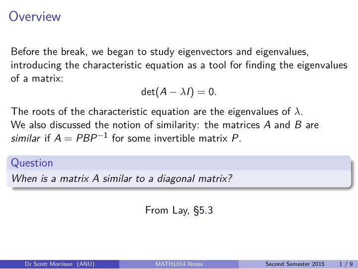
Overview Before the break, we began to study eigenvectors and eigenvalues, introducing the characteristic equation as a tool for finding the eigenvalues of a matrix: det( A − λ I ) = 0 . The roots of the characteristic equation are the eigenvalues of λ . We also discussed the notion of similarity: the matrices A and B are similar if A = PBP − 1 for some invertible matrix P . Question When is a matrix A similar to a diagonal matrix? From Lay, §5.3 Dr Scott Morrison (ANU) MATH1014 Notes Second Semester 2015 1 / 9

Quick review Definition An eigenvector of an n × n matrix A is a non-zero vector x such that A x = λ x for some scalar λ . The scalar λ is an eigenvalue for A . To find the eigenvalues of a matrix, find the solutions of the characteristic equation: det( A − λ I ) = 0 . The λ -eigenspace is the set of all eigenvectors for the eigenvalue λ , together with the zero vector. The λ -eigenspace E λ is Nul ( A − λ I ). Dr Scott Morrison (ANU) MATH1014 Notes Second Semester 2015 2 / 9

The advantages of a diagonal matrix Given a diagonal matrix, it’s easy to answer the following questions: 1 What are the eigenvalues of D ? The dimensions of each eigenspace? 2 What is the determinant of D ? 3 Is D invertible? 4 What is the characteristic polynomial of D ? 5 What is D k for k = 1 , 2 , 3 , . . . ? Dr Scott Morrison (ANU) MATH1014 Notes Second Semester 2015 3 / 9

The advantages of a diagonal matrix Given a diagonal matrix, it’s easy to answer the following questions: 1 What are the eigenvalues of D ? The dimensions of each eigenspace? 2 What is the determinant of D ? 3 Is D invertible? 4 What is the characteristic polynomial of D ? 5 What is D k for k = 1 , 2 , 3 , . . . ?  10 50  0 0 For example, let D = 0 π 0  .    0 0 − 2 . 7 Can you answer each of the questions above? Dr Scott Morrison (ANU) MATH1014 Notes Second Semester 2015 3 / 9

The diagonalisation theorem The goal in this section is to develop a useful factorisation A = PDP − 1 , for an n × n matrix A . This factorisation has several advantages: it makes transparent the geometric action of the associated linear transformation, and it permits easy calculation of A k for large values of k : Example 1   2 0 0 Let D = 0 − 4 0  .    0 0 − 1 Then the transformation T D scales the three standard basis vectors by 2 , − 4 , and − 1, respectively.  2 7  0 0 D 7 = ( − 4) 7 0 0  .    ( − 1) 7 0 0 Dr Scott Morrison (ANU) MATH1014 Notes Second Semester 2015 4 / 9

Example 2 � � 1 3 . We will use similarity to find a formula for A k . Suppose Let A = 2 2 � � � � 1 3 4 0 we’re given A = PDP − 1 where P = and D = . 1 − 2 0 − 1 We have PDP − 1 A = A 2 PDP − 1 PDP − 1 = Dr Scott Morrison (ANU) MATH1014 Notes Second Semester 2015 5 / 9

Example 2 � � 1 3 . We will use similarity to find a formula for A k . Suppose Let A = 2 2 � � � � 1 3 4 0 we’re given A = PDP − 1 where P = and D = . 1 − 2 0 − 1 We have PDP − 1 A = A 2 PDP − 1 PDP − 1 = PD 2 P − 1 = A 3 PD 2 P − 1 PDP − 1 = Dr Scott Morrison (ANU) MATH1014 Notes Second Semester 2015 5 / 9

Example 2 � � 1 3 . We will use similarity to find a formula for A k . Suppose Let A = 2 2 � � � � 1 3 4 0 we’re given A = PDP − 1 where P = and D = . 1 − 2 0 − 1 We have PDP − 1 A = A 2 PDP − 1 PDP − 1 = PD 2 P − 1 = A 3 PD 2 P − 1 PDP − 1 = PD 3 P − 1 = Dr Scott Morrison (ANU) MATH1014 Notes Second Semester 2015 5 / 9

Example 2 � � 1 3 . We will use similarity to find a formula for A k . Suppose Let A = 2 2 � � � � 1 3 4 0 we’re given A = PDP − 1 where P = and D = . 1 − 2 0 − 1 We have PDP − 1 A = A 2 PDP − 1 PDP − 1 = PD 2 P − 1 = A 3 PD 2 P − 1 PDP − 1 = PD 3 P − 1 = . . . . . . . . . A k PD k P − 1 = Dr Scott Morrison (ANU) MATH1014 Notes Second Semester 2015 5 / 9

So � � � � � � 4 k 1 3 0 2 / 5 3 / 5 A k = ( − 1) k 1 − 2 0 1 / 5 − 1 / 5 � 2 5 4 k + 3 3 5 4 k − 3 � 5 ( − 1) k 5 ( − 1) k = 5 4 k + 2 5 4 k − 2 2 3 5 ( − 1) k 5 ( − 1) k Dr Scott Morrison (ANU) MATH1014 Notes Second Semester 2015 6 / 9

Diagonalisable Matrices Definition An n × n (square) matrix is diagonalisable if there is a diagonal matrix D such that A is similar to D . That is, A is diagonalisable if there is an invertible n × n matrix P such that P − 1 AP = D ( or equivalently A = PDP − 1 ). Dr Scott Morrison (ANU) MATH1014 Notes Second Semester 2015 7 / 9

Diagonalisable Matrices Definition An n × n (square) matrix is diagonalisable if there is a diagonal matrix D such that A is similar to D . That is, A is diagonalisable if there is an invertible n × n matrix P such that P − 1 AP = D ( or equivalently A = PDP − 1 ). Question How can we tell when A is diagonalisable? The answer lies in examining the eigenvalues and eigenvectors of A . Dr Scott Morrison (ANU) MATH1014 Notes Second Semester 2015 7 / 9

Recall that in Example 2 we had � � � � � � 1 3 4 0 1 3 and A = PDP − 1 . A = , D = and P = 2 2 0 − 1 1 − 2 Note that � � � � � � � � 1 1 3 1 1 = = 4 A 1 2 2 1 1 and � � � � � � � � 3 1 3 3 3 = = − 1 . A − 2 2 2 − 2 − 2 Dr Scott Morrison (ANU) MATH1014 Notes Second Semester 2015 8 / 9

Recall that in Example 2 we had � � � � � � 1 3 4 0 1 3 and A = PDP − 1 . A = , D = and P = 2 2 0 − 1 1 − 2 Note that � � � � � � � � 1 1 3 1 1 = = 4 A 1 2 2 1 1 and � � � � � � � � 3 1 3 3 3 = = − 1 . A − 2 2 2 − 2 − 2 We see that each column of the matrix P is an eigenvector of A ... This means that we can view P as a change of basis matrix from eigenvector coordinates to standard coordinates! Dr Scott Morrison (ANU) MATH1014 Notes Second Semester 2015 8 / 9

In general, if AP = PD , then   λ 1 0 0 · · · 0 λ 2 0   · · · � � � �   = . A p 1 p 2 p n p 1 p 2 p n . . . · · · · · · ...   . . . . . .     0 0 λ n · · · � � If is invertible, then A is the same as p 1 p 2 p n · · ·   λ 1 0 0 · · · 0 λ 2 0 � − 1 .  · · ·  � � �   p 1 p 2 p n p 1 p 2 p n . . . ... · · · · · ·  . . .  . . .     0 0 λ n · · · Dr Scott Morrison (ANU) MATH1014 Notes Second Semester 2015 9 / 9