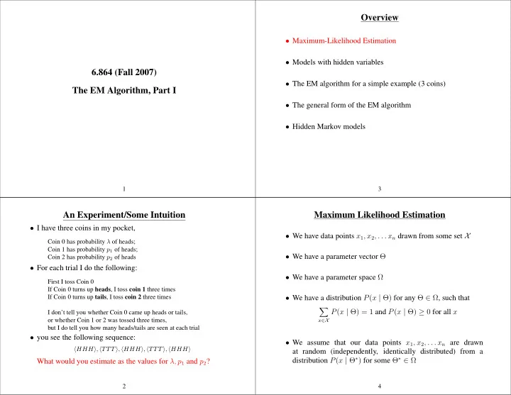
SLIDE 1 6.864 (Fall 2007) The EM Algorithm, Part I
1
An Experiment/Some Intuition
- I have three coins in my pocket,
Coin 0 has probability λ of heads; Coin 1 has probability p1 of heads; Coin 2 has probability p2 of heads
- For each trial I do the following:
First I toss Coin 0 If Coin 0 turns up heads, I toss coin 1 three times If Coin 0 turns up tails, I toss coin 2 three times I don’t tell you whether Coin 0 came up heads or tails,
- r whether Coin 1 or 2 was tossed three times,
but I do tell you how many heads/tails are seen at each trial
- you see the following sequence:
HHH, TTT, HHH, TTT, HHH
What would you estimate as the values for λ, p1 and p2?
2
Overview
- Maximum-Likelihood Estimation
- Models with hidden variables
- The EM algorithm for a simple example (3 coins)
- The general form of the EM algorithm
- Hidden Markov models
3
Maximum Likelihood Estimation
- We have data points x1, x2, . . . xn drawn from some set X
- We have a parameter vector Θ
- We have a parameter space Ω
- We have a distribution P(x | Θ) for any Θ ∈ Ω, such that
- x∈X
P(x | Θ) = 1 and P(x | Θ) ≥ 0 for all x
- We assume that our data points x1, x2, . . . xn are drawn
at random (independently, identically distributed) from a distribution P(x | Θ∗) for some Θ∗ ∈ Ω
4
SLIDE 2 Log-Likelihood
- We have data points x1, x2, . . . xn drawn from some set X
- We have a parameter vector Θ, and a parameter space Ω
- We have a distribution P(x | Θ) for any Θ ∈ Ω
- The likelihood is
Likelihood(Θ) = P(x1, x2, . . . xn | Θ) =
n
P(xi | Θ)
L(Θ) = log Likelihood(Θ) =
n
log P(xi | Θ)
5
A First Example: Coin Tossing
- X = {H,T}. Our data points x1, x2, . . . xn are a sequence of
heads and tails, e.g. HHTTHHHTHH
- Parameter vector Θ is a single parameter, i.e., the probability
- f coin coming up heads
- Parameter space Ω = [0, 1]
- Distribution P(x | Θ) is defined as
P(x | Θ) =
If x = H 1 − Θ If x = T
6
Maximum Likelihood Estimation
- Given a sample x1, x2, . . . xn, choose
ΘML = argmaxΘ∈ΩL(Θ) = argmaxΘ∈Ω
log P(xi | Θ)
- For example, take the coin example:
say x1 . . . xn has Count(H) heads, and (n − Count(H)) tails ⇒ L(Θ) = log
- ΘCount(H) × (1 − Θ)n−Count(H)
= Count(H) log Θ + (n − Count(H)) log(1 − Θ)
ΘML = Count(H) n
7
A Second Example: Probabilistic Context-Free Grammars
- X is the set of all parse trees generated by the underlying
context-free grammar. Our sample is n trees T1 . . . Tn such that each Ti ∈ X.
- R is the set of rules in the context free grammar
N is the set of non-terminals in the grammar
- Θr for r ∈ R is the parameter for rule r
- Let R(α) ⊂ R be the rules of the form α → β for some α
- The parameter space Ω is the set of Θ ∈ [0, 1]|R| such that
for all α ∈ N
Θr = 1
8
SLIDE 3
P(T | Θ) =
ΘCount(T,r)
r
where Count(T, r) is the number of times rule r is seen in the tree T
⇒ log P(T | Θ) =
Count(T, r) log Θr
9
Maximum Likelihood Estimation for PCFGs
log P(T | Θ) =
Count(T, r) log Θr
where Count(T, r) is the number of times rule r is seen in the tree T
L(Θ) =
log P(Ti | Θ) =
Count(Ti, r) log Θr
- Solving ΘML = argmaxΘ∈ΩL(Θ) gives
Θr =
- i Count(Ti, r)
- i
- s∈R(α) Count(Ti, s)
where r is of the form α → β for some β
10
Multinomial Distributions
- X is a finite set, e.g., X = {dog, cat, the, saw}
- Our sample x1, x2, . . . xn is drawn from X
e.g., x1, x2, x3 = dog, the, saw
- The parameter Θ is a vector in Rm where m = |X|
e.g., Θ1 = P(dog), Θ2 = P(cat), Θ3 = P(the), Θ4 = P(saw)
Ω = {Θ :
m
Θi = 1 and ∀i, Θi ≥ 0}
- If our sample is x1, x2, x3 = dog, the, saw, then
L(Θ) = log P(x1, x2, x3 = dog, the, saw) = log Θ1+log Θ3+log Θ4
11
Overview
- Maximum-Likelihood Estimation
- Models with hidden variables
- The EM algorithm for a simple example (3 coins)
- The general form of the EM algorithm
- Hidden Markov models
12
SLIDE 4 Models with Hidden Variables
- Now say we have two sets X and Y, and a joint distribution
P(x, y | Θ)
- If we had fully observed data, (xi, yi) pairs, then
L(Θ) =
log P(xi, yi | Θ)
- If we have partially observed data, xi examples, then
L(Θ) =
log P(xi | Θ) =
log
P(xi, y | Θ)
13
- The EM (Expectation Maximization) algorithm is a method
for finding ΘML = argmaxΘ
log
P(xi, y | Θ)
14
Overview
- Maximum-Likelihood Estimation
- Models with hidden variables
- The EM algorithm for a simple example (3 coins)
- The general form of the EM algorithm
- Hidden Markov models
15
The Three Coins Example
- e.g., in the three coins example:
Y = {H,T} X = {HHH,TTT,HTT,THH,HHT,TTH,HTH,THT} Θ = {λ, p1, p2}
P(x, y | Θ) = P(y | Θ)P(x | y, Θ) where P(y | Θ) = λ If y = H 1 − λ If y = T and P(x | y, Θ) = ph
1(1 − p1)t
If y = H ph
2(1 − p2)t
If y = T where h = number of heads in x, t = number of tails in x 16
SLIDE 5 The Three Coins Example
- Various probabilities can be calculated, for example:
P(x = THT, y = H | Θ) = λp1(1 − p1)2 P(x = THT, y = T | Θ) = (1 − λ)p2(1 − p2)2 P(x = THT | Θ) = P(x = THT, y = H | Θ) +P(x = THT, y = T | Θ) = λp1(1 − p1)2 + (1 − λ)p2(1 − p2)2 P(y = H | x = THT, Θ) = P(x = THT, y = H | Θ) P(x = THT | Θ) = λp1(1 − p1)2 λp1(1 − p1)2 + (1 − λ)p2(1 − p2)2
17
The Three Coins Example
- Various probabilities can be calculated, for example:
P(x = THT, y = H | Θ) = λp1(1 − p1)2 P(x = THT, y = T | Θ) = (1 − λ)p2(1 − p2)2 P(x = THT | Θ) = P(x = THT, y = H | Θ) +P(x = THT, y = T | Θ) = λp1(1 − p1)2 + (1 − λ)p2(1 − p2)2 P(y = H | x = THT, Θ) = P(x = THT, y = H | Θ) P(x = THT | Θ) = λp1(1 − p1)2 λp1(1 − p1)2 + (1 − λ)p2(1 − p2)2
18
The Three Coins Example
- Various probabilities can be calculated, for example:
P(x = THT, y = H | Θ) = λp1(1 − p1)2 P(x = THT, y = T | Θ) = (1 − λ)p2(1 − p2)2 P(x = THT | Θ) = P(x = THT, y = H | Θ) +P(x = THT, y = T | Θ) = λp1(1 − p1)2 + (1 − λ)p2(1 − p2)2 P(y = H | x = THT, Θ) = P(x = THT, y = H | Θ) P(x = THT | Θ) = λp1(1 − p1)2 λp1(1 − p1)2 + (1 − λ)p2(1 − p2)2
19
The Three Coins Example
- Various probabilities can be calculated, for example:
P(x = THT, y = H | Θ) = λp1(1 − p1)2 P(x = THT, y = T | Θ) = (1 − λ)p2(1 − p2)2 P(x = THT | Θ) = P(x = THT, y = H | Θ) +P(x = THT, y = T | Θ) = λp1(1 − p1)2 + (1 − λ)p2(1 − p2)2 P(y = H | x = THT, Θ) = P(x = THT, y = H | Θ) P(x = THT | Θ) = λp1(1 − p1)2 λp1(1 − p1)2 + (1 − λ)p2(1 − p2)2
20
SLIDE 6 The Three Coins Example
- Fully observed data might look like:
(HHH, H), (TTT, T), (HHH, H), (TTT, T), (HHH, H)
- In this case maximum likelihood estimates are:
λ = 3 5 p1 = 9 9 p2 = 0 6
21
The Three Coins Example
- Partially observed data might look like:
HHH, TTT, HHH, TTT, HHH
- How do we find the maximum likelihood parameters?
22
The Three Coins Example
- Partially observed data might look like:
HHH, TTT, HHH, TTT, HHH
- If current parameters are λ, p1, p2
P(y = H | x = HHH) = P(HHH, H) P(HHH, H) + P(HHH, T) = λp3
1
λp3
1 + (1 − λ)p3 2
P(y = H | x = TTT) = P(TTT, H) P(TTT, H) + P(TTT, T) = λ(1 − p1)3 λ(1 − p1)3 + (1 − λ)(1 − p2)3
23
The Three Coins Example
- If current parameters are λ, p1, p2
P(y = H | x = HHH) = λp3
1
λp3
1 + (1 − λ)p3 2
P(y = H | x = TTT) = λ(1 − p1)3 λ(1 − p1)3 + (1 − λ)(1 − p2)3
- If λ = 0.3, p1 = 0.3, p2 = 0.6:
P(y = H | x = HHH) = 0.0508 P(y = H | x = TTT) = 0.6967
24
SLIDE 7 The Three Coins Example
- After filling in hidden variables for each example,
partially observed data might look like: (HHH, H) P(y = H | HHH) = 0.0508 (HHH, T) P(y = T | HHH) = 0.9492 (TTT, H) P(y = H | TTT) = 0.6967 (TTT, T) P(y = T | TTT) = 0.3033 (HHH, H) P(y = H | HHH) = 0.0508 (HHH, T) P(y = T | HHH) = 0.9492 (TTT, H) P(y = H | TTT) = 0.6967 (TTT, T) P(y = T | TTT) = 0.3033 (HHH, H) P(y = H | HHH) = 0.0508 (HHH, T) P(y = T | HHH) = 0.9492
25
The Three Coins Example
(HHH, H) P(y = H | HHH) = 0.0508 (HHH, T) P(y = T | HHH) = 0.9492 (TTT, H) P(y = H | TTT) = 0.6967 (TTT, T) P(y = T | TTT) = 0.3033 . . . λ = 3 × 0.0508 + 2 × 0.6967 5 = 0.3092 p1 = 3 × 3 × 0.0508 + 0 × 2 × 0.6967 3 × 3 × 0.0508 + 3 × 2 × 0.6967 = 0.0987 p2 = 3 × 3 × 0.9492 + 0 × 2 × 0.3033 3 × 3 × 0.9492 + 3 × 2 × 0.3033 = 0.8244
26
The Three Coins Example: Summary
- Begin with parameters λ = 0.3, p1 = 0.3, p2 = 0.6
- Fill in hidden variables, using
P(y = H | x = HHH) = 0.0508 P(y = H | x = TTT) = 0.6967
- Re-estimate parameters to be λ = 0.3092, p1 = 0.0987, p2 =
0.8244
27 Iteration λ p1 p2 ˜ p1 ˜ p2 ˜ p3 ˜ p4 0.3000 0.3000 0.6000 0.0508 0.6967 0.0508 0.6967 1 0.3738 0.0680 0.7578 0.0004 0.9714 0.0004 0.9714 2 0.4859 0.0004 0.9722 0.0000 1.0000 0.0000 1.0000 3 0.5000 0.0000 1.0000 0.0000 1.0000 0.0000 1.0000 The coin example for y = {HHH, TTT, HHH, TTT}. The solution that EM reaches is intuitively correct: the coin-tosser has two coins, one which always shows up heads, the other which always shows tails, and is picking between them with equal probability (λ = 0.5). The posterior probabilities ˜ pi show that we are certain that coin 1 (tail-biased) generated y2 and y4, whereas coin 2 generated y1 and y3. 28
SLIDE 8
Iteration λ p1 p2 ˜ p1 ˜ p2 ˜ p3 ˜ p4 ˜ p5 0.3000 0.3000 0.6000 0.0508 0.6967 0.0508 0.6967 0.0508 1 0.3092 0.0987 0.8244 0.0008 0.9837 0.0008 0.9837 0.0008 2 0.3940 0.0012 0.9893 0.0000 1.0000 0.0000 1.0000 0.0000 3 0.4000 0.0000 1.0000 0.0000 1.0000 0.0000 1.0000 0.0000 The coin example for {HHH, TTT, HHH, TTT, HHH}. λ is now 0.4, indicating that the coin-tosser has probability 0.4 of selecting the tail-biased coin. 29 Iteration λ p1 p2 ˜ p1 ˜ p2 ˜ p3 ˜ p4 0.3000 0.3000 0.6000 0.1579 0.6967 0.0508 0.6967 1 0.4005 0.0974 0.6300 0.0375 0.9065 0.0025 0.9065 2 0.4632 0.0148 0.7635 0.0014 0.9842 0.0000 0.9842 3 0.4924 0.0005 0.8205 0.0000 0.9941 0.0000 0.9941 4 0.4970 0.0000 0.8284 0.0000 0.9949 0.0000 0.9949 The coin example for y = {HHT, TTT, HHH, TTT}. EM selects a tails-only coin, and a coin which is heavily heads-biased (p2 = 0.8284). It’s certain that y1 and y3 were generated by coin 2, as they contain heads. y2 and y4 could have been generated by either coin, but coin 1 is far more likely. 30 Iteration λ p1 p2 ˜ p1 ˜ p2 ˜ p3 ˜ p4 0.3000 0.7000 0.7000 0.3000 0.3000 0.3000 0.3000 1 0.3000 0.5000 0.5000 0.3000 0.3000 0.3000 0.3000 2 0.3000 0.5000 0.5000 0.3000 0.3000 0.3000 0.3000 3 0.3000 0.5000 0.5000 0.3000 0.3000 0.3000 0.3000 4 0.3000 0.5000 0.5000 0.3000 0.3000 0.3000 0.3000 5 0.3000 0.5000 0.5000 0.3000 0.3000 0.3000 0.3000 6 0.3000 0.5000 0.5000 0.3000 0.3000 0.3000 0.3000 The coin example for y = {HHH, TTT, HHH, TTT}, with p1 and p2 initialised to the same value. EM is stuck at a saddle point 31 Iteration λ p1 p2 ˜ p1 ˜ p2 ˜ p3 ˜ p4 0.3000 0.7001 0.7000 0.3001 0.2998 0.3001 0.2998 1 0.2999 0.5003 0.4999 0.3004 0.2995 0.3004 0.2995 2 0.2999 0.5008 0.4997 0.3013 0.2986 0.3013 0.2986 3 0.2999 0.5023 0.4990 0.3040 0.2959 0.3040 0.2959 4 0.3000 0.5068 0.4971 0.3122 0.2879 0.3122 0.2879 5 0.3000 0.5202 0.4913 0.3373 0.2645 0.3373 0.2645 6 0.3009 0.5605 0.4740 0.4157 0.2007 0.4157 0.2007 7 0.3082 0.6744 0.4223 0.6447 0.0739 0.6447 0.0739 8 0.3593 0.8972 0.2773 0.9500 0.0016 0.9500 0.0016 9 0.4758 0.9983 0.0477 0.9999 0.0000 0.9999 0.0000 10 0.4999 1.0000 0.0001 1.0000 0.0000 1.0000 0.0000 11 0.5000 1.0000 0.0000 1.0000 0.0000 1.0000 0.0000 The coin example for y = {HHH, TTT, HHH, TTT}. If we initialise p1 and p2 to be a small amount away from the saddle point p1 = p2, the algorithm diverges from the saddle point and eventually reaches the global maximum. 32
SLIDE 9 Iteration λ p1 p2 ˜ p1 ˜ p2 ˜ p3 ˜ p4 0.3000 0.6999 0.7000 0.2999 0.3002 0.2999 0.3002 1 0.3001 0.4998 0.5001 0.2996 0.3005 0.2996 0.3005 2 0.3001 0.4993 0.5003 0.2987 0.3014 0.2987 0.3014 3 0.3001 0.4978 0.5010 0.2960 0.3041 0.2960 0.3041 4 0.3001 0.4933 0.5029 0.2880 0.3123 0.2880 0.3123 5 0.3002 0.4798 0.5087 0.2646 0.3374 0.2646 0.3374 6 0.3010 0.4396 0.5260 0.2008 0.4158 0.2008 0.4158 7 0.3083 0.3257 0.5777 0.0739 0.6448 0.0739 0.6448 8 0.3594 0.1029 0.7228 0.0016 0.9500 0.0016 0.9500 9 0.4758 0.0017 0.9523 0.0000 0.9999 0.0000 0.9999 10 0.4999 0.0000 0.9999 0.0000 1.0000 0.0000 1.0000 11 0.5000 0.0000 1.0000 0.0000 1.0000 0.0000 1.0000 The coin example for y = {HHH, TTT, HHH, TTT}. If we initialise p1 and p2 to be a small amount away from the saddle point p1 = p2, the algorithm diverges from the saddle point and eventually reaches the global maximum. 33
Overview
- Maximum-Likelihood Estimation
- Models with hidden variables
- The EM algorithm for a simple example (3 coins)
- The general form of the EM algorithm
- Hidden Markov models
34
The EM Algorithm
- Θt is the parameter vector at t’th iteration
- Choose Θ0 (at random, or using various heuristics)
- Iterative procedure is defined as
Θt = argmaxΘQ(Θ, Θt−1) where Q(Θ, Θt−1) =
P(y | xi, Θt−1) log P(xi, y | Θ)
35
The EM Algorithm
- Iterative procedure is defi ned as Θ
t = argmaxΘQ(Θ, Θt−1), where
Q(Θ, Θt−1) =
P(y | xi, Θt−1) log P(xi, y | Θ)
– Intuition: fi ll in hidden variables y according to P(y | x
i, Θ)
– EM is guaranteed to converge to a local maximum, or saddle-point,
- f the likelihood function
– In general, if argmaxΘ
log P(xi, yi | Θ) has a simple (analytic) solution, then argmaxΘ
P(y | xi, Θ) log P(xi, y | Θ) also has a simple (analytic) solution. 36
SLIDE 10 Overview
- Maximum-Likelihood Estimation
- Models with hidden variables
- The EM algorithm for a simple example (3 coins)
- The general form of the EM algorithm
- Hidden Markov models
37
The Structure of Hidden Markov Models
- Have N states, states 1 . . . N
- Without loss of generality, take N to be the final or stop state
- Have an alphabet K. For example K = {a, b}
- Parameter πi for i = 1 . . . N is probability of starting in state i
- Parameter ai,j for i = 1 . . . (N − 1), and j = 1 . . . N is
probability of state j following state i
- Parameter bi(o) for i = 1 . . . (N −1), and o ∈ K is probability
- f state i emitting symbol o
38
An Example
- Take N = 3 states. States are {1, 2, 3}. Final state is state 3.
- Alphabet K = {the, dog}.
- Distribution over initial state is π1 = 1.0, π2 = 0, π3 = 0.
- Parameters ai,j are
j=1 j=2 j=3 i=1 0.5 0.5 i=2 0.5 0.5
- Parameters bi(o) are
- =the
- =dog
i=1 0.9 0.1 i=2 0.1 0.9
39
A Generative Process
- Pick the start state s1 to be state i for i = 1 . . . N with
probability πi.
- Set t = 1
- Repeat while current state st is not the stop state (N):
– Emit a symbol ot ∈ K with probability bst(ot) – Pick the next state st+1 as state j with probability ast,j. – t = t + 1
40
SLIDE 11 Probabilities Over Sequences
- An output sequence is a sequence of observations o1 . . . oT
where each oi ∈ K e.g. the dog the dog dog the
- A state sequence is a sequence of states s1 . . . sT where each
si ∈ {1 . . . N} e.g. 1 2 1 2 2 1
- HMM defines a probability for each state/output sequence pair
e.g. the/1 dog/2 the/1 dog/2 the/2 dog/1 has probability π1 b1(the) a1,2 b2(dog) a2,1 b1(the) a1,2 b2(dog) a2,2 b2(the) a2,1 b1(dog)a1,3 Formally:
P(s1 . . . sT , o1 . . . oT ) = πs1× T
P(si | si−1)
T
P(oi | si)
41
A Hidden Variable Problem
- We have an HMM with N = 3, K = {e, f, g, h}
- We see the following output sequences in training data
e g e h f h f g
- How would you choose the parameter values for πi, ai,j, and
bi(o)?
42
Another Hidden Variable Problem
- We have an HMM with N = 3, K = {e, f, g, h}
- We see the following output sequences in training data
e g h e h f h g f g g e h
- How would you choose the parameter values for πi, ai,j, and
bi(o)?
43